Chalmers Advanced Python
Lab 2: Graphs and transport networks
Advanced Python Course
Chalmers DAT690 / DIT516 / DAT516
2025
by Aarne Ranta & John J. Camilleri
Purpose
The purpose of this lab is to build a system of classes and algorithms for graphs. The intended application is transport networks, which will be built on top of the graph classes. But the graphs can be applied in many other ways as well, as will be shown in exercises and extra labs.
The main learning outcomes are:
- Python’s data model for classes
- class definitions with private instance variables, public methods, and “hidden” methods
- inheritance between classes
- understanding and extending an external library, the
networkxlibrary - representations of graphs
- Dijkstra’s shortest path algorithm with different cost functions
- visualization of graphs and paths in them, using the
graphvizlibrary - property-based testing with randomized input data, using the
hypothesislibrary
Overview
You are expected to submit four Python files:
graphs.pyimplementing general graphs and graph algorithmstrams.pyimplementing transport networks by using concepts fromgraphs.pytest_graphs.pycontaining tests for the code ingraphs.pytest_trams.pycontaining tests for the code intrams.py
The following UML diagram shows the classes that you are expected to implement in these files.
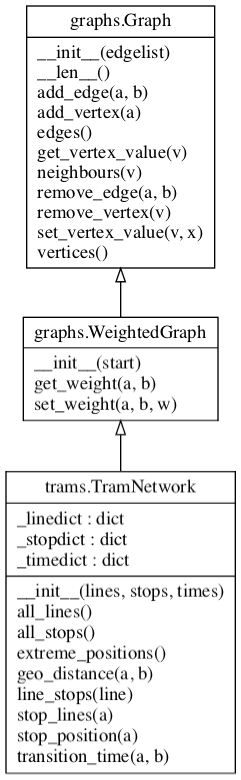
The underscored instance variables shown above are just hints that need not be followed. The important thing is that the public methods are implemented with the names given here.
In addition to these classes, you will have to implement the following functions:
# in graphs.py
dijkstra(graph, source, cost=lambda u,v: 1)
visualize(graph, view='view', name='mygraph', nodecolors={})

# in trams.py
readTramNetwork(tramfile=TRAM_FILE)
The functionalities of these classes and functions will be specified in detail below.
Last but not least, you will have to write tests using either the unittest or hypothesis libraries, or both.
Task 1: file graphs.py
The Graph class
The class Graph represents an undirected graph, built of vertices and edges, where the vertices can have values associated with them.
Rather than implement everything from scratch, we will reuse many features from the networkx library. In order to add our own functionality and tailor the API to our liking, we define our own Graph class which will inherit and reuse the networkx implementation internally.
Constructor
The class can be initialized in two ways:
- from
None(the default) - from a list of edges
The implementation is by inheritance from networkx.Graph:
import networkx as ns

class Graph(nx.Graph):
    def __init__(self, start=None):
        super().__init__(start)
Note that the start argument of nx.Graph() can be a list of edges, as required in this lab, but it can also be other things, such as an adjacency list.
The class internally builds a data structure that supports different graph operations.
This data structure is kept hidden, and it is inherited from the Graph class of the networkx library, so you don’t need to define any hidden instance variables.
Methods
The public methods needed are:
neighbors(vertex): return an iterator over all vertices adjacent tovertexvertices(): return all vertices in the graphedges(): return all edges in the graph (undirected)__len__(): return the number of verticesadd_vertex(vertex): addvertexto the graphadd_edge(vertex1, vertex1): add an edge betweenvertex1andvertex2remove_vertex(vertex): removevertexfrom graph and all edges to itremove_edge(vertex1, vertex2): remove edge betweenvertex1andvertex2, but not the vertices (even if left unconnected)get_vertex_value(vertex): return the value ofvertexset_vertex_value(vertex, value): set the value ofvertextovalue
Some of the public methods required above already exist in nx.Graph with exactly the same names.
They do not need to be defined in your class, since they are inherited.
Some other methods have different names, so to implement the desired API you have to write, for example:
def vertices(self):
    return self.nodes()
Vertex values
The trickiest part is perhaps the values of vertices. In the tram network, for example, they can be used to store information such as the location of a tram stop.
In networkx, values are stored in dictionaries associated with the nodes themselves.
Here is a minimal example suggesting how you could set and get values of nodes:
>>> G = nx.Graph()
>>> G.add_node(9)
>>> G.nodes[9]['value'] = 234
>>> G.nodes[9]
{'value': 234}
The vertex values can initially be None.
The WeightedGraph class
WeightedGraph is a subclass of Graph, which stores edge weights.
These weights can be objects of any type.
In the tram network, for instance, they can store transition times between adjacent stops.
The class supports two additional public methods:
get_weight(vertex, vertex)set_weight(vertex, vertex, weight)
Since Graph is implemented by inheritance from networkx, you can
implement these methods by using the representation of weights that is
already available there:
>>> G = nx.Graph()
>>> G.add_edge(1,2)
>>> G[1][2]['weight'] = 8
>>> G[1][2]['weight']
8
The shortest path algorithm
Next, we want to implement the function:
dijkstra(graph, source, cost=lambda u,v: 1)
which computes the shortest path from the source vertex to all other vertices, as a dictionary.
It should return the paths as sorted lists of vertices, including the source and the target.
What is shortest is calculated by the minimum sum of the cost function applied to each step on the path.
For example, if graph is a WeightedGraph, its get_weight() method can be used.
But any function that takes two vertex arguments is possible, for instance, their geographical distance (which is calculated from vertex values rather than stored for each edge, to avoid redundancy).
Using the networkx implementation
The networkx implementation of Dijkstra’s algorithm is the function:
shortest_path(graph, source=None, target=None, weight=None, method='dijkstra')
which you can call in your own dijkstra function.
To do so, you:
- pass the
graphandsourcearguments tonx.shortest_path, - leave out the
target, thus causing the function to produce a dictionary for all targets, - convert the
costfunction to aweightattribute, - leave out the
method, so that the default is used.
The tricky part is the conversion of cost in our code (which is a function) to weight in the networkx implementation (which is an attribute of edges).
The following helper function can be used for this purpose:
def costs2attributes(G, cost, attr='weight'):
    for a, b in G.edges():
        G[a][b][attr] = cost(a, b)
For comparison: a native implementation
If you want to understand the details of dijkstra, you can follow the pseudocode in
this Wikipedia article.
Make sure to return a dictionary, where the keys are all target vertices reachable from the source, and their values are paths from the source to the target (i.e. lists of vertices in the order that the shortest path traverses them).
Notice that the Wikipedia pseudocode algorithm does not return the paths.
But they can be constructed inside the same algorithm when the dist dictionary is updated: this dictionary should not only contain the distances, but also the paths, and the path can be updated at the same time as the distance.
(Notice also that the networkx function always returns the paths.)
Visualization
A very simple visualization function is expected in Lab 2; we will make it more sophisticated in Lab 3. The function you must implement is:
visualize(graph, view='view', name='mygraph', nodecolors=None)
For this we will use the Graphviz library.
Note that apart from installing the Python package graphviz, you will also need to install the Graphviz program on your computer and make sure it is in your system’s PATH.
The description in the lecture notes is simple but sufficient for this function, except for how to use nodecolors, which you should look up in the Graphviz library documentation.
The view parameter can be used with the following values:
view='view': a window with the graph picture is popped up (by callingrender(view=True)ingraphviz)view='pdf': just generate a pdf file without opening it (callrender()without arguments)
The main intended use of nodecolors is to show the nodes along the shortest path in a different colour.
To try this out, you can use the following code:
def view_shortest(G, source, target, cost=lambda u,v: 1):
    path = dijkstra(G, source, cost)[target]
    print(path)
    colormap = {str(v): 'orange' for v in path}
    print(colormap)
    visualize(G, view='view', nodecolors=colormap)

def demo():
    G = Graph([(1,2),(1,3),(1,4),(3,4),(3,5),(3,6),(3,7),(6,7)])
    view_shortest(G, 2, 6)

if __name__ == '__main__':
    demo()
Testing your graph implementation
You will need to implement some test for your graphs module in the file test_graphs.py.
We recommend the use of the hypothesis library, but this is a recommendation rather than a requirement.
Here are some things to test:
- if
(a, b)is inedges(), bothaandbare invertices() - if
ahasbas its neighbour, thenbhasaas its neighbour - the shortest path from
atobis the reverse of the shortest path frombtoa(but notice that this can fail in situations where there are several shortest paths)
When grading your lab, we will check that your test file test_graphs.py contains some reasonable tests and shows that you are able to use the test libraries.
However, we will also run our own tests on your graphs.py file.
If we then find errors, you may have to resubmit your lab.
To prevent this from happening, we recommend that you take your own testing seriously!
Task 2: file trams.py
This file needs to import two of your own modules:
graphs.pyfrom Lab 2tramdata.pyfrom Lab 1
The standard sys library is needed if you have your Lab 1 solution in a different directory (which we recommend).
If so you need to tell Python where to find the file tramdata.py as follows:
import sys
sys.path.append('../lab1/')
import tramdata as td
The TramNetwork class
The class TramNetwork is a WeightedGraph (i.e. inherits from it) where:
- the vertices are all the stops
- the edges are transitions between consecutive stops on some line
- the weights are the transition times between adjacent stops
The internals of this class can be implemented using the dictionaries for lines, stops, and times from Lab 1.
The public methods that we need are getters for:
- the position of a stop
- the transition time between two subsequent stops
- the geographical distance between any two stops (from Lab 1)
- list the lines through a stop (just the line numbers, or whole objects)
- list the stops along a line (just the stop names, or whole objects)
- list all stops (just the stop names, or whole objects)
- list all lines (just the line numbers, or whole objects)
If you use the names suggested in the UML diagram, some things in Lab 3 will be easier.
Notice that you need not store geographical distances between stops, because they can be computed from the positions of stops. For this, you can use the geographical distance function from Lab 1.
Finally, the class should have a extreme_positions() method which should return the minimum and maximum latitude and longitude found among all stop positions.
Reading a TramNetwork
The JSON file tramnetwork.json produced in Lab 1 contains all the information needed for building an instance of TramNetwork.
The function:
readTramNetwork(tramfile=TRAM_FILE)
should do exactly this, defaulting to tramnetwork.json, which should however be given via the global variable TRAM_FILE.
It should return an object of class TramNetwork.
Remember that you will need to import the standard json library to parse JSON files.
Testing trams.py
Some of the tests from Lab 1 are also relevant here, now performed on the TramNetwork class and its methods.
You can try to generate data for them from the stop and line lists by using hypothesis.
Another thing to test is the connectedness of the tram network. This could be done simply by just depth-first or breadth-first search.
The following demo is also a good test for yourself: if you see that it works flawlessly, you can be fairly sure that all parts of your code work as they should.
Demo
You can paste the following code to your trams.py file to demonstrate and test it:
def demo():
    G = readTramNetwork()
    a, b = input('from,to ').split(',')
    view_shortest(G, a, b)

if __name__ == '__main__':
    demo()
When you run the code, it asks you to enter two tram stop names separated by a comma (no spaces between). It then displays the whole tram network, with the shortest path (as the number of stops) coloured.
Submission
You should submit the following files:
graphs.pytrams.pytest_graphs.pytest_trams.py