Chalmers Advanced Python
Lecture Notes for the Continuation Course in Python
Aarne Ranta, John J. Camilleri, Muhammad Mustafa Hassan
Preface
This guide is written for the students of the continuation course in Python at Chalmers University of Technology and University of Gothenburg. The original name of the course was “Advanced Programming in Python”, starting in 2021. As of 2024, the course name is “Continuation Course in Programming in Python”, which reflects better its character as an intermediate rather than an advanced course.
The purpose of this guide is to give a unified view of the course and help your learning by showing the big picture and pointing you to further reading. It is not a complete description of the course material: we found it unnecessary, and even harmful, to repeat and digest all the material that you are expected to read. On the advanced level of programming, you should be able to read the original documentation, which you can find on the internet, and which may be difficult or even confusing. This guide will help you to get started, by giving pointers to material that we found relevant and which you at least should read while studying this course.
Table of contents
- 1. Introduction
- 2. Learning the Python language
- 3. Diving into the official tutorial
- 3.1. Tutorial 1: Whetting your appetite
- 3.2. Tutorial 2: Using the Python interpreter
- 3.3. Tutorial 3: An informal introduction to Python
- 3.4. Tutorial 4: More control flow tools
- 3.5. Tutorial 5: Data structures
- 3.6. Tutorial 6: Modules
- 3.7. Tutorial 7: Input and Output
- 3.8. Tutorial 8: Errors and Exceptions
- 3.9. Tutorial 9: Classes
- 3.10. Tutorial 10 and 11: the Standard Library
- 3.11. Tutorial 12: Packages and virtual environments
- 3.12. Tutorial 13: What Now?
- 4. Storing and retrieving information
- 5. Graphs and graph algorithms
- 6. Object-oriented design
- 7. Testing
- 8. Visualization
- 9. Web programming
- 10. The rest of Python
- A. Appendix: Git version control system
1. Introduction
1.1. The aims of this guide and the course
This course is a second course in programming, after an introduction course. After learning the basics of programming, the ambition here is to reach a level of completeness:
- Complete knowledge of Python: you will know all constructs of the Python language, not only the ones covered by introduction courses.
- Universal programming potential: you will get the confidence that you can solve any programming task, as just a matter of having enough time to study the problem and work on it.
The latter goal is related to the idea of a computer as a universal machine, which is able to perform all tasks that an algorithm can do. What is needed for this is, in addition to the peripheral devices, a programmer that can implement those algorithms on the machine. The goal of this course is to help you to become that programmer.
Really to become an advanced programmer, you will also need to learn some other things. This includes courses that are more specific than just programming: they will cover topics such as data structures and algorithms, machine learning, and software engineering. Even more importantly, you will have to develop your skills by programming in practice. Another name for the “universal programmer” is full-stack developer. This means a programmer that masters all levels of a practical application. The term is often used more specifically to mean a web application consisting of a back end, database, and a front end. This course is centered around a programming project where you will build a full-stack web an application.
1.2. Programmers of different kinds
This course is mainly targeted to bachelor-level students, who have studied an introductory Python course. But it was originally designed, and is still available for, students from different backgrounds - computer science, data science, mathematics, physics, chemistry, design, engineering, business, ecology - and levels - bachelor, masters, PhD. Many of the mentioned fields have their own cultures of programming. It is helpful to identify some of them, because you are likely to meet these cultures during your future programmer career. The following three profiles are of course caricatures, but you can easily find code examples that satisfy all characteristics in each of them.
1.2.1. The Computer Scientist
This is the context in which the course is formally given. In this context, programming is a branch evolved from applied mathematics. The programmer is interested in the mathematical structure of programs and tries to find the most elegant data structures and algorithms. She also wants to make them as general and abstract as possible. Her programs are typically not solutions to practical problems, but more on the level of libraries that can be used by others who are solving practical problems. The hard-core computer scientist programmer does not primarily use libraries herself - instead, she tries to understand and build everything from the first principles.
Here are some typical features of the Computer Scientist’s programs:
- they consist of functions whose size is just a few lines each,
- each function has a clear mathematical description,
- they are often close to pseudocode that could be published in a textbook,
- variable and function names are often short and similar to ones used in mathematics,
- the code avoids language-specific idioms,
- classes are used mainly to define data structures - not to structure entire programs,
- the code is accompanied by arguments about correctness and complexity,
- the code is not tested thoroughly, just demoed with a couple of examples if not proved correct,
- there are very few comments in the code, since it is aimed to be self-explanatory,
- the programs are written by single persons and are self-contained.
With the growing needs of computer programs, Computer Scientist programmers are becoming more and more of a minority. They have, to some extent, made themselves superfluous by creating libraries that other programmers can rely on and do not need to understand the internals of. But of course, they are needed in the front line of research to invent new algorithms, new programming languages, and new kinds of computing devices. It is also common that theoretical Computer Science questions are used in interviews at tech companies.
1.2.2. The Software Engineer
This category contains the majority of programmers who have programming as their profession. They typically have a Computer Science background, but have “grown up” from that when getting encountered with the “real world”. They have learned several programming languages and have lots of algorithms and data structures in their “toolbox”. At the same time they know that, to solve a practical problem or to create end-user software, no single technique is sufficient in itself. They have no time to go into the internals of algorithms, but use whatever libraries and tools they - or their managers - have learned to trust. They often work in large groups and try to maintain a level of readability that enables others in the group take over their code.
Here are some typical features of the Software Engineer’s programs:
- they are divided into modules and classes with complex hierarchies,
- each unit of the program is documented in detail with comments and often with diagrams,
- the names of variables, functions, and classes are long, descriptive, and systematic,
- the code is accompanied by a comprehensive set of tests,
- the code uses libraries whenever possible, avoiding to “reinvent the wheel”,
- the code has a long lifetime and may have ancient layers that no-one dares to touch any more,
- the full software system may have code written in many languages and typically also contains configuration files and build scripts.
Competent software engineers on different domains of application are constantly and increasingly wanted by employers. Their competence may be based on academic education, but it is primarily a product of years of experience. It is not proven by academic degrees or publications, but by a portfolio of software that the programmer has designed or contributed to. This experience often comes from enterprises, but it can also be built in open source projects where the programmer has made major contributions.
1.2.3. The Occasional Programmer
This is the category of programmers with no or little training in Computer Science. They can be teenagers or other hobby programmers, but also proficient scientist or engineers in other disciplines, who see programming as something that can be learned in an afternoon or two, when it is needed for some computations or experiments. For scientists, programming is a replacement of the earlier use of pencil and paper for similar tasks (now decades ago). Computers make it faster to apply mathematical formulas, and they make it feasible to deal with larger amounts of data than in earlier times, in particular if statistics or machine learning is involved.
Typical features of programs in this category are:
- the structure of the code is simple and linear - in Python, this means that it consists of top-level statements and global variables, avoiding functions and classes,
- the program is a single file that can be thousands of lines long,
- variable names are short and unsystematic,
- input and output is performed freely in different places of the code,
- as there are no return statements, the only way to combine the code with other programs is to pipe its output to them as a string,
- the code uses freely whatever libraries seem to do the job,
- libraries are often imported in the middle of the file rather than in the beginning,
- the code is written by one person and is not intended even to be read by others,
- the code does one thing, aiming to do it with as little effort as possible,
- the code is only run once or a few times,
- well, it is often run with the same input a large number of times, until it seems to do the job in the expected way,
- if a related task appeared again, the code is copied and patched to fit for that purpose.
This category of programmers is probably the largest, and includes both professionals and hobby programmers. In fact, since Python supports this style so well, it is occasionally used by all kinds of programmers. Programs in this category are often called scripts rather than “real programs”. If you search the web for a Python solution to a particular problem, you are likely to find several examples of this kind of code: scripts with linear structure where large blocks are copies of each other and where input and output happen all over the place.
1.2.4. Programming in this course
The main part of this course belongs to the Software Engineer category:
- we want to solve substantial practical problems,
- we use proven techniques and libraries for this,
- we structure the code in a clear and reusable way,
- we document the code in a way that explains it to other programmers,
- we raise the level of reliability of the code by systematic testing.
As a support for this, we will also look into some Computer Science topics:
- the data model and semantics of Python,
- some fundamental algorithms and their theoretical aspects.
We will neither cover nor recommend the Occasional Programmer’s style, not even for highly competent professionals in advanced scientific fields. If you are a scientist, you are probably right if you think that programming is easy compared with the deeper questions you deal with in your actual research. But even then, we believe that it is helpful to learn about the algorithms and data structures of the computer scientist, as well as the techniques and practices of the software engineer. This can make you both faster and more confident when writing code for your next experiment.
One can also compare programming with other hobbies: almost anyone can learn to cook food or play an instrument without any formal training or even without reading books that teach these skills. But if you take your hobby seriously, it will give you more satisfaction if you know that you are doing it “the right way”.
1.3. The Lab
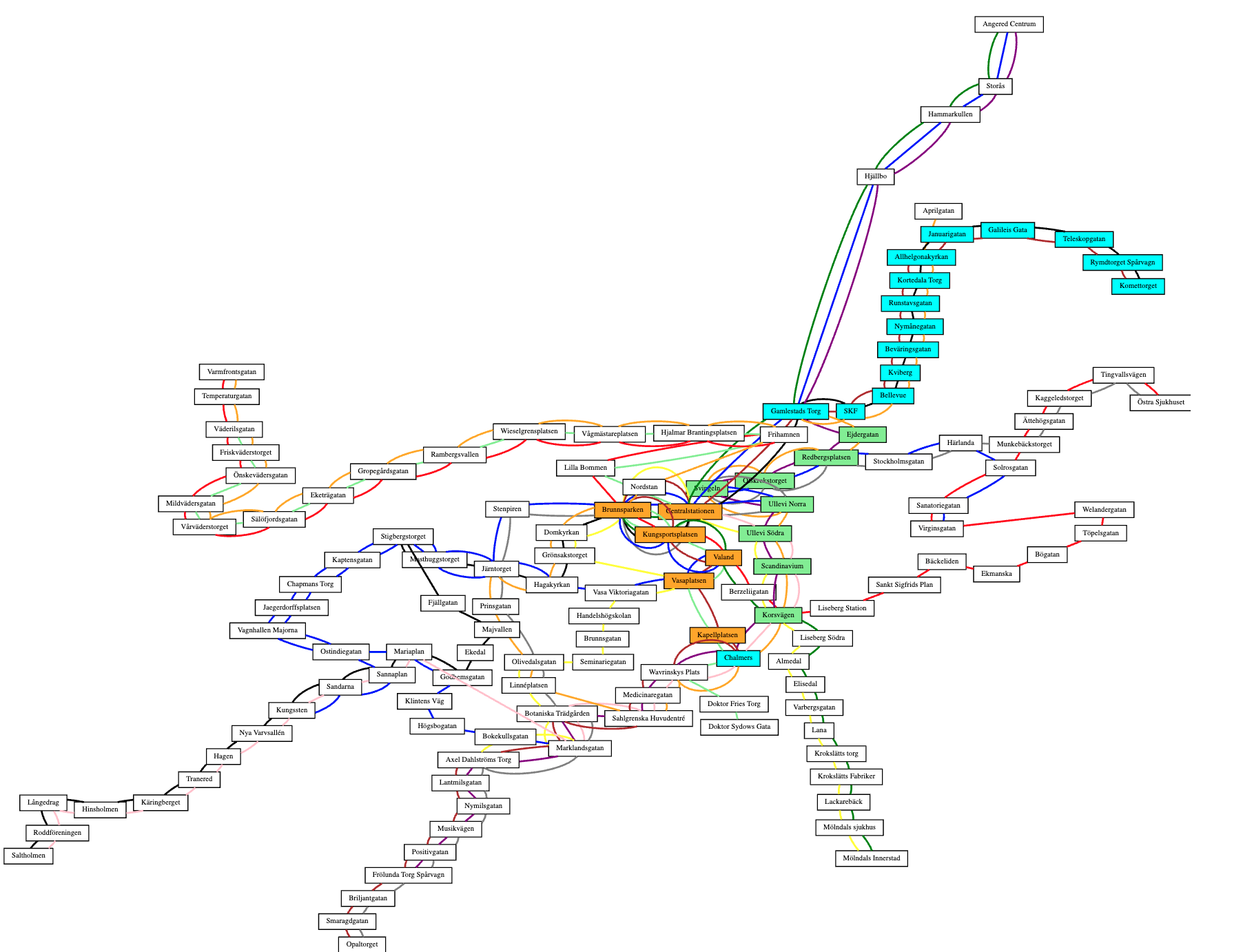
Much of the course is centered around the Lab, a programming assignment whose goal is to build a “full-stack” web application. In the final demonstration of the application, the user can search for a route in the Gothenburg tram network and get it drawn on a map - in the way familiar from the numerous travel planning applications on the web. The Lab is described in detail in three parts (Lab 1, Lab 2, and Lab 3) so let us here just explain the purpose of the lab in the context of the course.
The Lab is primarily an exercise in practical Software Engineering and serves the following learning outcomes:
- to write modular, well structured programs with reusable components,
- to use standard libraries and understand their documentation,
- to apply testing and version control practices,
- to read and peer review code written by others,
- to document program code so that it can be understood by others,
- to get the basics of some useful techniques (graphs, visualization, web programming) that can be applied to numerous other tasks.
In addition, the Lab has some Computer Science aspects:
- to learn about graphs, which are a fundamental concept in many computing tasks,
- to widen your imagination so that you can search for solutions to practical problems from well-known general algorithms.
The title page of this document shows a screen dump of the final web application.
The standard Lab was in earlier course instances extended with a couple of related tasks, which use graphs for other things than route finding. They can be found in the “old-labs” directory of the course repository, in case you want to try your hand with them:
- map colouring: making sure that neighbouring countries have different colours,
- machine learning: finding clusters (tightly connected parts) in a network.
The basic lab is estimated to require up to two weeks of working time in total. The actual time consumption is individual and depends greatly on your previous experience.
2. Learning the Python language
One goal of the course is to bring you to a level where they have seen “all of Python”. This does not yet mean that you can use all constructs of Python efficiently. But you will have at least heard about things like dictionaries, slicing, comprehensions, decorators, inheritance, dunder methods, and other special constructs that might not be familiar from your previous programming language.
2.1. What do I learn when I learn a language
Computer scientists and software engineers typically know several programming languages. They are also comfortable in learning new ones. Actually, if you are young (say, under 40), it is unlikely that Python will be the language of choice during the rest of your remaining professional life. Likewise, for most of us over 40 at least, Python is not our first programming language, but it can be, for instance, Java or Haskell or C or Pascal.
When learning your second or third programming language, you certainly do not need to learn everything that absolute beginners are taught their first programming language. You only need, so to say, learn the differences between the new language and your earlier ones.
The situation resembles learning a second language when you already know your native language - for instance, learning English when you already know Swedish. It has probably taken you at least seven years to learn to speak, read, and write Swedish fluently. You have had to learn not only what words mean which things, but also the very idea that words can stand for things, and that written signs can represent sounds. While learning this, your brain and motoric skills have developed to use a language. If you start learning English at this point, most of this infrastructure is already in place. Therefore, it is not uncommon to learn a new language fairly well in a couple of months, which is totally unconceivable when a child learns its first language.
So let us assume, analogously to Java programmers learning Python, that you are a native speaker of Swedish beginning to learn English. You know that the language consists of words, which are combined to phrases and sentences. What you need to learn is
- syntax: how phrases and sentences are formed,
- vocabulary: what words are used for what things.
In many cases, learning the syntax of a new language is a task that can be completed in a couple of weeks, since it will not be very different from your earlier languages. You will learn, for instance, that negation in English is formed in a different way from Swedish, by using auxiliary verbs (I don’t know instead of I know not). It might take longer to use actively all parts of the syntax, but you will at least understand the structure of what you read, even if you need to look up words in a dictionary.
The vocabulary, in contrast to syntax, involves life-long learning. Even native speakers may occasionally need to look up a word in a dictionary.
Now, when learning Python on top of Java (or any other programming language on top of any other one), it is a good idea to start with the syntax - more precisely, how its syntax differs from Java, “how negation is expressed in Python” (yes, it uses the keyword not instead of the operator !).
Most of this will be fairly obvious and follow a handful of general rules, while some things have no counterparts in Java.
At the same time, some things available in Java are not available in Python, and for those things you will have to learn to express them in a different way.
Within a week or so - Python syntax is a lot easier than English - you will be able to understand the syntactic structure of everything that is written in Python. There may be things you will never use in your own code, and will probably have a bias for Java-like expression - just like Swedish native speakers, even when fluent in English, can be biased to Swedish-like constructs.
In this course, we will actually try to help you become more Pythonic, since this will give you some satisfaction as well as credibility among Pythonistas. But I must confess that, since my own “native” programming language is not Python, I cannot guarantee always to be Pythonic myself.
What about the vocabulary of Python? There are 35 reserved words (“keywords”), and they are quickly learned as a part of the syntax. In addition, there are 68 built-in functions, many of which you will not need any time soon. But the main bulk of the vocabulary is in library functions and classes, and they involve life-long learning. The only viable approach is to learn to “look up words in the dictionary”, that is, search for class and function names in library documentation.
2.2. Some characteristics of Python syntax
2.2.1. Modules, classes, functions, statements
Assuming that your first language is Java, you have probably started with a “Hello World” program like this one:
class Hello {
    public static void main(String args[]){
        System.out.println("Hello World");
    }
}
In order to run it, you have first compiled it to Java bytecode with the ‘javac’ program, and then executed the resulting binary with the ‘java’ program:
$ javac Hello.java
$ java Hello
Hello World
If you mechanically convert your Java program into Python code, you will get
class Hello:
    def main():
        print("Hello World")

Hello.main()
In order to run this, you just need to run ‘python’ (often named ‘python3’ to distinguish it from earlier versions):
$ python3 hello.py
Hello World
In other words, there is no separate step of compilation, but you can “run your program directly”. (In reality, there is a compilation phase to Python’s bytecode, but it happens behind the scenes.) Thus running the code is simpler, but the code itself is about as complicated as in Java.
However, the code shown above is what you end up with if you directly convert your Java thinking into Python. The “normal” Hello World program in Python is much simpler:
print("Hello World")
This program consists of a single statement - no class, no function is needed. There is also an intermediate way to write the same program, which contains a function but no class:
def main():
    print("Hello World")

main()
If your background is in C or Haskell rather than Java, this will probably be the most natural way to write the Hello World program.
The Hello World examples illustrate the different levels in which programs are structured in both Java and Python, and also in many other languages:
- modules (typically files),
- classes,
- functions (or “methods”),
- statements,
- expressions.
In Java, these levels are strictly nested: expressions reside inside statements, statements inside functions, functions inside classes, and classes are the top-level structure of modules. In Python, the same strict hierarchy can be followed, but this is not compulsory. It is common that a top-level module is a mixture of classes, functions, and statements. An extreme case is a module consisting only of statements: this is the dominating style in what we called “occasional programming” and has given Python the label “scripting language”.
Even though we will discourage code consisting of top-level statements, we have to add that Python in fact does not even force any nesting of the levels: class and function definitions are themselves statements, and can appear anywhere inside other statements, such as the bodies of while loops.
Hence, if you want to write ten times “Hello World”, you can do it as follows:
i = 0

while i < 10:
    class Hello:
        def main():
            print("Hello World")
    Hello.main()
    i += 1
This, of course, is not good use of the freedom you get in Python. It is overly complicated to write, as well as overly expensive to run (because extra code is generated under the hood every time a class or a function is defined). But we will later see situations where functions inside functions, or even classes inside functions, are a good way to write programs.
2.2.2. The layout syntax
Both Java and C programmers are used to terminating statements with semicolons (;) and enclosing blocks of code in curly brackets ({}).
This is not the case in Python (nor in Haskell).
Instead,
- statements are terminated by newlines,
- blocks are marked by adding indentation.
As a general rule,
- a line ending with a colon (
:) marks the beginning of a new block, expecting added indentation on the next line, - these lines start with a keyword such as
class,def,while, - a block ends when indentation comes back to some of the earlier levels.
A slight modification in these rules is that it is possible to divide a statement, or a line expecting a new block to start, into several lines.
In that case, one also has either to end each line but the last with a backslash \ or be inside the scope of an open parenthesis or bracket.
Thus all of the following are permitted:
x = 6 +\
7
x = (6 +
7)
xs = [6,
7]
Such examples are, however, rare and typically appear only if the lines contain expressions that are two long to fit into the recommended 79 characters per line - for example, long lists or dictionaries.
And yes, indeed, Python comes with recommended lengths for lines and indentations:
- lines should not be longer than 79 characters,
- each indentation level should be 4 spaces (no tabs recommended),
- each class and function definition should be separated by 2 blank lines.
Such rules may sound pedantic at first, but if you follow them, they will soon become a second nature and make your Python code easier to read.
2.2.3. Dynamic typing
Another thing that Python is known for is the lack of types in code:
- function definitions do not indicate argument or return types,
- variable types are not declared.
The lack of types in Python source code is sometimes taken to mean that “Python has no types”. But this is not true: Python does not have types of expressions, but it does have types of their values, i.e. objects that are created at run time, when the program is executed. Hence the correct term to use is dynamic typing.
Dynamic typing implies that there is no static type checking of your source code. An expression - such as a variable or a function call - can have different types in different places in code, and even at different runs of the program. It can then happen that no possible type is found, which leads to a run-time type error.
A statically typed language such as Java can find type errors at compile time and prevent the execution of the program. This is not provided by Python: it can in fact happen that a program is run 1000 times without failures, but after that a type error is encountered when the execution, for the first time, enters a rarely used branch of some conditional. Thus it is difficult ever to be sure that your Python program is failure-free.
What is more, the lack of static checking does not only concern types, but also function and variable names. If a name in a rare branch has a typo, making it into a name that is not in scope, you will only notice this when some run of the program enters this branch.
Some later extensions of Python have made it possible to equip functions type annotations, and there are programs that perform static type checking. This is not yet standard, but it is increasingly used, and we will introduce some of it during this course to tell the complete story of Python. Static type annotations are particularly useful in the documentation of code, especially function type signatures. But they are deemed to be incomplete, because Python is intended to support a high degree of polymorphism. This means that functions can be applied to many different types, and it is difficult to specify in advance which types these exactly are. Type information in library documentation is often - particularly in older libraries - given in natural language rather than as type annotations.
2.3. A grammar of Python
This section is something you can just glance through and use later as reference. The main purpose at this point is to show that there is not so much language-wise you need to learn: just a couple of pages. We will explain most of the things in more detail when going through the tutorial.
Our grammar is a condensed and somewhat simplified version of the official grammar in
https://docs.python.org/3/reference/grammar.html
We show the syntax of Python in the BNF notation (Backus-Naur form). While the grammar covers slightly less than the full grammar, its shortness is mainly due to its higher level of abstraction. In particular, it does not indicate precedence levels, which regulate the evaluation order and the use of parentheses.
<stm> ::= <decorator>* class <name> (<name>,*)?: <block>
        | <decorator>* def <name> (<arg>,*): <block>
        | import <name> <asname>?
        | from <name> import <imports>
        | <exp>,* = <exp>,*
        | <exp> <assignop> <exp>
        | for <name> in <exp>: <block>
        | <exp>
        | return <exp>,*
        | yield <exp>,*
        | if <exp>: <block> <elses>?
        | while <exp>: <block>
        | pass
        | break
        | continue
        | try: <block> <except>* <elses> <finally>?
        | assert <exp> ,<exp>?
        | raise <name>
        | with <exp> as <name>: <block>
<decorator> ::= @ <exp>
<asname>    ::= as <name>
<imports>   ::= * | <name>,*
<elses>     ::= <elif>* else: <block>
<elif>      ::= elif exp: <block>
<except>    ::= except <name>: <block>
<finally>   ::= finally: <block>
<block>     ::= <stm> <stm>*
<exp> ::= <exp> <op> <exp>
        | <name>.?<name>(<arg>,*)
        | <literal>
        | <name>
        | ( <exp>,* )
        | [ <exp>,* ]
        | { <exp>,* }
        | <exp>[exp]
        | <exp>[<slice>,*]
        | lambda <name>*: <exp>
        | { <keyvalue>,* }
        | ( <exp> for <name> in <exp> <cond>? )
        | [ <exp> for <name> in <exp> <cond>? ]
        | { <exp> for <name> in <exp> <cond>? }
        | - <exp>
        | not <exp>
<keyvalue> ::= <exp>: <exp>
<arg> ::= <name>
        | <name> = <exp>
        | *<name>
        | **<name>
<cond> ::= if <exp>
<op>  ::= + | - | * | ** | / | // | % | @
        | == | > | >= | < | <= | !=
        | in | not in | and | or
<assignop> ::= += | -= | *=
<slice> ::= <exp>? :<exp>? <step>?
<step>  ::= :<exp>?
Here are the reserved words, each of which also appears in the above grammar:
and as assert break class continue def del elif else except False finally for from global import if in is lambda None not or pass raise return True try while with yield
The literals are infinite classes of “words”, the most important of which are:
-
strings: enclosed in single quotes
'...', double quotes"...", or multiple lines between groups of three quotes"""...""", -
integers: any number of digits
1234567890, -
floats: digits with decimal point and possibly with exponent indicating powers of ten
3.14,.005,2.9979e8,6.626e-34,
Comments are lines starting with #.
A comment can also terminate a non-comment line, but it is recommended to use entire lines.
Multi-line comments can be given as string literals in triple quotes """, which is also a common way to “comment out” longer pieces of code.
To conclude the explanation of words, the following built-in functions will appear throughout the course:
abs(x)absolute value of a number,bool(x)conversion from various types to booleans,chr(n)conversion from numeric code to character,dict(c?)creation of or conversion to a dictionary,dir(m)listing of contents in a module,eval(s)evaluation of a string as an expression,exec(s)execution of a string as a statement,float(x)conversion to a float,help(f)documentation of a function, class, or module,input(p='')receiving input from promptp,init(x)conversion to integer,len(c)length of a collection,list(x?)creation of or conversion to list,max(c)maximum of a collection,min(c)minimum of a collection,next(g)receive the next object from a generator,open(f)open a file,ord(c)numeric code of a character,print(x*)print a sequence of objects,range(m=0, n), range of integers frommton-1,reversed(s)reverse of a sequence,round(d, p=0), round a float topdecimals,set(c?)creation of or conversion to a set,sorted(s)sorting a sequence,str(x)conversion to a string,sum(c)sum of a collection,super()superclass of a class,tuple(c?)create or convert to a tuple,type(x)type of an object.
The tutorial will cover many of these in more detail. A full list, with full details, can be found at:
https://docs.python.org/3/library/functions.html
In addition to the built-in functions, there are several methods for built-in classes that are used all the time. Here are some:
- strings:
split(),join(),format(),index(), - lists:
append(),sort(),reverse(),pop(), - dictionaries:
get(),keys(),values(),items(), - sets:
add(),remove().
The on-line help in the Python shell is always available for more information. For instance, the command:
help(str)
gives a detailed list of all methods available for strings.
3. Diving into the official tutorial
This chapter goes through the official Python tutorial in:
https://docs.python.org/3/tutorial/index.html
by showing some highlights from it. The tutorial is written by the creator of Python, Guido van Rossum. It covers practically everything in the Python language, and does it in a way that makes you hear van Rossum’s line of thought when designing the language. Hence it is recommended reading from the beginning to the end. However, it is not a tutorial for beginner programmers, but assumes - just like we are doing here - that you already know the basic concepts from some other context.
3.1. Tutorial 1: Whetting your appetite
There is one point we want to raise: the chapter says that “Python also offers much more error checking than C”. This is not completely true, because C has static type checking and Python does not. In C - as in many other languages - static type checking is needed to support compilation to bare machine code (as opposed to virtual machine code in the case of Python). In processors such as Intel and ARM, different instructions and registers are used for different types of objects, e.g. for integers and floating point numbers. To make an optimal use of the machine, one has to know the types of expressions at compile time.
Static typing and compilation to machine code is what makes languages like C to enable more efficient programs than Python. This is because Python programs, when executed by a computer, must eventually use the machine code instructions of the computer. The execution of virtual machine code needs several times more instructions than if the same algorithm was directly available in real machine code. Much of this is, however, helped by enabling Python code to use modules written in C via a foreign code interface. Many of the standard functions and methods, e.g. for lists and dictionaries, are ultimately written in C. Using them whenever possible is therefore not only easier but also more efficient than writing your own algorithms over lists and dictionaries.
3.2. Tutorial 2: Using the Python interpreter
This chapter explains the different ways of invoking the Python interpreter. The main options are:
- running the entire program from the operating system shell (in a way familiar from Java and C),
- opening the Python shell and importing the module from there (familiar from e.g. Lisp, Haskell, and Prolog).
From the operating system shell
You can write
$ python3 hello.py
where the source file name is given, or
$ python3 -m hello
where the module name (without extension .py) is given.
We will return to the use of command line arguments (sys.argv[]) when discussing the sys library.
Inside the Python shell
First start the Python shell from the operating system, then import the module from there.
$ python3
[welcome message displayed]
>>> import hello
You will then be able to execute statements that refer to functions and classes defined in hello.py:
>>> hello.hello()
Hello World
You can of course execute statements that do not refer to the imported module. This you can do even without importing any module:
$ python3

>>> print(2+2)
4
What is more, you can evaluate expressions in the shell, so that their values are shown, without the need of print() around.
>>> 2+2
4
This is a difference between writing code in the shell and in Python files: if you write just 2+2 on a line in a Python file, nothing is shown about it when you run the module. To see the value, you must make the expression into a statement by using print().
The shell has two kinds of prompts:
>>>, the primary prompt, corresponding to no indentation in a Python file,..., the secondary prompt, expecting added indentation.
The secondary prompt is needed when you for instance want to run a for loop in the shell:
>>> for i in range(2):
...     print("Yes!")
...
Yes!
Yes!
You must remember to add the indentation and keep it constant. An empty line will get you back to level 0.
To my personal taste, it is quite awkward to write multiline statements in a shell, and therefore I prefer writing them inside functions in files and just calling these functions from the shell.
If you import hello from the Python shell, you can access the functions in it with the prefix hello..
You can avoid this by writing, instead,
>>> from hello import *
Then all names defined on the top level of the file become available without a prefix. This is handy if you open the file in the purpose of testing its functions in different combinations.
The effect of both ways of importing a module is that the statements in it are executed in the order in which they appear.
This can be disturbing, if you are for instance opening a module in order to test the functions in it one by one.
You can avoid most of the disturbance by not including print() statements on the top level but only inside functions - which is a good practice anyway.
A more general way to restrict the statements to use from command lines is to run them under the condition
if __name__ == '__main__':
    # statements executed only when used from command line
3.3. Tutorial 3: An informal introduction to Python
Numbers
Here are some points of interest, potentially surprising:
- Integers have arbitrary size, whereas floats have limited precision. Therefore, int to float conversion can be lossy:
>>> int(float(12345678901234567890))
12345678901234567168
Notice that the type names int and float are themselves used as conversion functions.
- The floor division operator
//returns the largest integer smaller than the floating point value; its absolute value can be different depending on the sign of the result:
>>> 20 // 7
2

>>> -20 // 7
-3
Strings
Points of interest:
-
Single and double quotes mean the same; an advantage is that escapes of quotes are seldom needed:
'"Yes," they said.' -
Evaluating a string literal shows quotes (usually converted to single), printing it drops the quotes:
>>> 'hello' 'hello' >>> "hello" 'hello' >>> 'hello' == "hello" True >>> print('hello') hello -
Notice also that there is a type difference.
NoneTypeis used for expressions that return no useful value, such as those formed byprint(). To see the type, you can use thetype()function:>>> type('hello') <class 'str'> >>> type(print('hello')) hello <class 'NoneType'> -
Raw strings prefixed with
rtreat backslashes literally:>>> print('\tmp\name') mp ame >>> print(r'\tmp\name') \tmp\nameIn normal string literals,
\tis tab and\nis newline, as shown above. -
Triple quotes
"""enclose multiple line string literals. This is also the way to create multiline comments - or comment out blocks of code. -
Two or more string literals are glued together:
>>> 'Py' 'thon' 'Python' -
You can concatenate strings with
+and multiply by*:>>> name = 'Joe' >>> 'hey ' + name 'hey Joe' >>> 6*name 'JoeJoeJoeJoeJoeJoe' -
Notice that
print()takes many arguments, converts all to strings, and adds spaces:>>> print(name, 23, 'years') Joe 23 yearsBut
+requires explicit conversions and spaces:>>> name + 23 + 'years' TypeError: can only concatenate str (not "int") to str >>> name + str(23) + 'years' 'Joe23years' -
The index notation
[]returns characters in given positions, starting from 0. A negative index counts backwards from the last character, -1.>>> 'hello'[0] 'h' >>> 'hello'[4] 'o' >>> 'hello'[-1] 'o'Notice that there is no special type of characters: a character is simply a one-character string.
-
The slice notation generalizes from the index notation to substrings.
  >>> 'hello'[1:4]
  'ell'
Notice that the first index is included, the second one is not: slices is like a semi-open intervals in mathematics, in this case
[1,4[. -
The start and end indices in slices are optional:
>>> 'hello'[:2] 'he' >>> 'hello'[2:] 'llo' -
Adding a third argument indicates a step
  >>> '0123456789'[0:9:2]
  '02468'
Quiz: you can create the reverse of a string by using negative indices and steps. How?
The final point in this section is that strings are immutable. Mutability is a general topic, which we will cover when comparing strings with lists.
Lists
Points of interest:
-
Lists can be given with the bracket notation, and indexed and sliced just like strings:
>>> digits = [0, 1, 2, 3, 4, 5, 6, 7, 8, 9] >>> digits[6] 6 >>> digits[3:6] [3, 4, 5] -
One can assign values to indices, as lists are mutable
  >>> digits[4] = 'four'
  >>> digits
  [0, 1, 2, 3, 'four', 5, 6, 7, 8, 9]
Notice here also that a list can contain elements of different types.
-
You can also assign lists to slices - even lists of a different size:
>>> digits[3:5] = ['III','IV'] >>> digits [0, 1, 2, 'III', 'IV', 5, 6, 7, 8, 9] >>> digits[3:5] = [] >>> digits [0, 1, 2, 5, 6, 7, 8, 9] -
Unlike lists, strings are not mutable. To create a “mutable string”, you can make a copy that is converted to a list, and join the result back to a string:
  >>> s = 'python'
  >>> ls = list(s)
  >>> ls
  ['p', 'y', 't', 'h', 'o', 'n']

  >>> ls[0] = 'P'
  >>> ls
  ['P', 'y', 't', 'h', 'o', 'n']

  >>> ''.join(ls)
  'Python'
This is a useful technique when lots of changes are performed on a long string, because using lists instead of strings avoids creating new copies of the string.
First steps towards programming
The Fibonacci example
a, b = 0, 1

while a < 10:
    print(a)
    a, b = b, a+b
shows a while loop, which is probably familiar, but also two examples of a multiple assignment - assignment to several variables simultaneously.
A simple standard example of multiple assignment is swapping the values of two variables:
a, b = b, a
Without multiple assignments, doing this would require a temporary third variable.
3.4. Tutorial 4: More control flow tools
Loops and conditionals
Many of the statement forms for control flow are familiar from other languages, with just minor differences:
whileloops (above, from Tutorial 3.2),if-elif-elsestatements, which can have any number ofelifbranches,forloops, which can iterate over any iterable type (such lists and strings, but dictionaries and sets),breakstatements, which interrupt a loop and go back to the previous block level,continuestatements, which interrupt a loop and go to the next round of iteration,returnstatements anywhere in a function body terminates the execution of the function and returns the value of the expression given in the statements, orNoneif no expression is included.
Some statement forms are less familiar:
passstatements, which do nothing - commonly used as place-holders for what would be an empty block in a language using brackets,matchstatements, starting from Python 3.10, which enable structural pattern matching familiar from functional languages such as Haskell.
Of the familiar statements, for loops provide a prime example of what is considered “Pythonic”, that is, coding style that maximally uses the possibilities of Python.
Here is an example: a for loop that simply prints each character of a string:
for c in s:
    print(c)
A less Pythonic way go get the same output is to loop over an index that ranges from 0 to the length of the string:
for i in range(len(s))
    print(s[i])
This style is considered overly complicated, except if you really need to access the integer index. An example of this is if you want to print every second letter of a string:
for i in range(len(s))
    if i%2 == 0:
        print(s[i])
The range() function, by the way, creates sequences of integers,
- the sequence 0,1,2,3,4 for
range(5) - the sequence 2,3,4 for
range(2,5)
The function len() returns the length of a list or a string.
Another example where looping over an index is needed is the following: if you want to change a list, for instance increment each element in it by one, you might try
ds = [1, 2, 3, 4]

for d in ds:
    d += 1
But this will not change the list ds.
What it does is just to give new values to the variable d.
The proper way to increment each element in the list is to assign to each element of it:
for i in range(len(ds)):
    ds[i] += 1
One more thing: you might expect that the variable bound in the for loop has its scope limited to that loop.
But in fact, the variable continues to be alive, with the last value assigned to it in the loop.
Hence for instance i has the value 3 after the loop just shown.
This is different from many other programming languages, where variables declared in compound statements have their scopes only within those statements.
The match statement (Tutorial 4.6) is a novelty in Python 3.10.
It will look familiar to functional programmers - and it actually feels like the missing piece to some of us! - but we will cover it only later in these lecture notes, when we make sure that we have explained every detail of Python’s syntax.
Function definitions
Function definitions, as observed before, have no type information attached to the parameters or to the return values.
This makes it possible to define functions that return different types of values, or nothing at all (which in Python, however, is treated as value None), in different branches of a conditional.
An example is the following function that finds floating point roots for quadratic equations
import math

def quadratic_eq(a, b, c):

    discr = b**2 - 4*a*c

    if discr < 0:
        print("no roots")
    elif discr == 0:
        return -b/(2*a)
    else:
        rdiscr = math.sqrt(discr)
        return [(-b - rdiscr)/(2*a),
                (-b + rdiscr)/(2*a)]
A problem with this style is that it is difficult for another function to take the output of this function as input. For instance, it cannot loop over the roots, because the result is iterable (a list) only if there are two roots. In this case, it would of course be easy to make each of the three branches return a list.
The number of arguments to a function can be varied by using optional arguments that have, if not given, default values:
def ask_ok(prompt, retries=4, reminder='Please try again!'):
The first argument is a positional arguments, which is compulsory to give. The other arguments can be given either by position or by using the variable name, then known as keyword arguments. The order of keyword arguments is not significant, but they must come after the positional arguments:
ask_ok('> ', 3)    # third arg 'Please try again'
ask_ok('> ', reminder='Come on!')  # second arg 4
ask_ok('> ', reminder='Come on!', retries=3)
Yet another specialty of Python is the use of packed arguments, marked by
*for any list (or tuple) of positional arguments,**for any list of keyword arguments
which must appear in this order, as in the Tutorial example
def cheeseshop(kind, *arguments, **keywords):
The markers / and * used as in
def f(pos1, pos2, /, pos_or_kwd, *, kwd1, kwd2):
are yet another way specify how arguments can be passed to a function. Tutorial Section 4.8.3.5 (in version 3.10) gives guidance for how to use this mechanism in the intended way.
Lambda expressions
Lambda expressions create anonymous functions - functions that are created without defining them with def statements.
A common use is in keyword arguments, for instance, in sorting:
>>> pairs = [(1, 'one'), (2, 'two'), (3, 'three'), (4, 'four')]
>>> pairs.sort(key=lambda pair: pair[1])
>>> pairs
[(4, 'four'), (1, 'one'), (3, 'three'), (2, 'two')]
An alternative to this would be:
def snd(pair):
    return pair[1]

pairs.sort(key=snd)
The point with using lambda is that a line of code is saved and no name is needed for this function that is used only once. A limitation is that the definition of the lambda function must be single expression, hence it cannot contain statements.
Documentation strings and function annotations
A string literal immediately after a function header (the def line), as in:
def quadratic_eq(a, b, c):
    "solving quadratic equations"
    # etc
has a special status as a documentation string.
It gives the value of the “invisible” __doc__ variable, but also the answer to the help() function:
>>> quadratic_eq.__doc__
'solving quadratic equations'

>>> help(quadratic_eq)

Help on function quadratic_eq in module mymath:

quadratic_eq(a, b, c)
    solving quadratic equations
Including documentation strings is a good practice, in particular in library functions. They can consist of many lines if triple quotes are used.
Functions can also be equipped with annotations (Tutorial 4.8.8) that give type information. They can be useful for documentation, but, unlike in e.g. Java, they are not checked by the compiler, and their expressivity is limited. For example, if a function has variable argument and return types, there is no standard way to express this.
Coding style
We have already mentioned then “Pythonic” recommendations to use 4 spaces for indentation 2 empty lines between functions, and maximum line length 79 characters. Some others are mentioned here, and we will try to follow them, in particular:
- spaces after commas, e.g.
f(x, y), lowercase_with_underscoresfor function names.
In many other languages, camelCase is preferred for function names, which makes it natural to continue this convention in Python.
However, this will soon lead to mixtures of the two conventions when libraries are used, which gives a messy impression.
3.5. Tutorial 5: Data structures
This section covers different types of collections:
- lists, e.g.
[1, 4, 9] - dictionaries, e.g.
{'computer': 'dator', 'language': 'språk'} - tuples, e.g.
'computer', 'dator'(parentheses not needed!) - sets, e.g.
{1, 4, 9}
To these, one could also add two kinds of sequences that we have already seen:
- strings, e.g.
hello - ranges, e.g.
range(1,101)
These six types have a lot in common, but also differences that make them usable for different purposes. Therefore it is often necessary to convert between them, and we will cover some of the main ways to do so. The conversions sometimes work as expected, but sometimes lead to loss of information. Thus converting a list of tuples into a dictionary keeps both components of tuples, but converting a dictionary into a list only keeps the keys:
>>> dict([(1, 2)])
{1: 2}

>>> list({1: 2})
[1]
Notice, however, that converting a list with several values given to the same keys results in a dictionary that only includes the last of the values:
>>> dict([(1, 2), (1, 5)])
{1: 5}
The fundamental explanation of all differences lies in a handful of hidden methods in class definitions, which we will cover in the chapter on the data model of Python. The visible part of these concepts can be seen in type error messages, such as:
>>> s = "hello"
>>> s[3] = 'c'
TypeError: 'str' object does not support item assignment
You should go through all of the methods listed in the official Tutorial 5.1, not only for lists but also for the other data structures, to get a feeling of which of them work for which.
Notice that all of the collections mentioned in this section are objects of classes, which have methods applied by using a special syntax - for instance,
xs.sort()
which is really a shorthand for a function application
list.sort(xs)
In other words, the object xs is really the first argument of the function sort()from the class list.
Normally, the first variant, the object-oriented notation is recommended for these functions.
Comprehensions
List comprehensions are introduced in the official tutorial 5.1.3, and provide a powerful, highly Pythonic way to create lists from given ones via the operations of mapping and filtering.
Mapping is the transformation of every item in a list in a certain way, for example squaring a list of numbers. This can be done using a simple for loop:
numbers = [1,2,3,4,5]
squares = []
for n in numbers:
    squares.append(n**2)
Using a list comprehension this can be expressed as:
>>> [ n**2 for n in numbers ]
[1, 4, 9, 16, 25]
Filtering is selecting a subset of items from a list based on some predicate, for example filtering out the even numbers:
evens = []
for n in numbers:
    if n % 2 == 0:
        evens.append(n)
Using a list comprehension this can be expressed as:
>>> [ n for n in numbers if n % 2 == 0 ]
[2, 4]
Furthermore, list comprehensions allow us to map and filter together, for example building a list of squares of even numbers:
>>> [ n**2 for n in numbers if n % 2 == 0 ]
[4, 16]
What gives even more power is that comprehensions work for other collection types as well, and even for mixtures of them. Thus we have dictionary comprehensions,
>>> {n: n**3 for n in range(7)}
{0: 0, 1: 1, 2: 8, 3: 27, 4: 64, 5: 125, 6: 216, 7: 343}
and set comprehensions
>>> {n % 3 for n in range(100)}
{0, 1, 2}
We will make heavy use of comprehensions as a query language for structured data in Chapter 4.
Booleans
There are a couple of special things about booleans:
-
Keywords
and,or,notare used for boolean operators. -
Comparison operators can be chained:
a < b <= cmeans the same asa < b and b <= c. -
Many types can be cast into booleans:
0,'',[],{}all count asFalsewhen used in conditions. -
Boolean
orcan return values in these other types:>>> {} or 0 or 'this' 'this' >>> {} or 0 0 -
Finally, let us tell you a secret that is not covered by the tutorial: Python has a conditional expressions, which have a slightly surprising syntax:
  >>> x = 10
  >>> 'big' if x > 10 else 'small'
  'small'
Thus the “true” value comes first, the condition in the middle, and the “false” value last.
A summary of collection types
| type | notation | indexing | assignment | mutable | order | reps |
|---|---|---|---|---|---|---|
str |
'hello' |
s[2] |
- | no | yes | yes |
list |
[1, 2, 1] |
l[2] |
l[2] = 8 |
yes | yes | yes |
tuple |
(1, 2, 1) |
t[2] |
- | no | yes | yes |
dict |
{'x': 12} |
d['x'] |
d['x'] = 9 |
yes | no | no |
set |
{1, 2} |
- | - | yes | no | no |
range |
range(1,7) |
r[2] |
- | no | yes | no |
The difference between lists and sets is the familiar one from mathematics: lists care about the order of elements, and remember repetitions of elements (“reps” in the table), whereas sets store every element just ones and does not specify their order. Hence the order in which a set is converted to a list can be different from the order in which the set was defined:
>>> s = {4, 1, 2}
>>> list(s)
[1, 2, 4]
This also explains why indexing with position does not work for sets.
Dictionaries function as sets in two respects: order and repetitions. But unlike sets, they allow indexing via keys (the things on the left sides of the colons).
The ordering is illustrated by how equality works. The following tests show that order matters for lists but not for sets:
>>> [2, 3] == [3, 2]
False

>>> {2, 3} == {3, 2}
True
What about dictionaries? A new implementation in Python 3.6 is reported to preserve the order in which the items are introduced; see https://docs.python.org/3.6/whatsnew/3.6.html.
However, this does not change the mathematical property that order is irrelevant (tested in 3.9.7):
>>> {1: 2, 2: 3} == {2: 3, 1: 2}
True
Mutability and item assignment go hand in hand, except for sets, where indexing makes no sense.
But sets are still mutable, by the add() and remove() methods:
>>> s = {4, 1, 2}
>>> s.add(8)
>>> s
{8, 1, 2, 4}
>>> s.remove(2)
>>> s
{8, 1, 4}
3.6. Tutorial 6: Modules
3.6.1. Importing
Modules can be imported from both the Python shell and from Python files in many different ways:
-
import mathmakesmath.cos(), math.sin()available -
import math as mmakesm.cos(), m.sin()available -
from math import cosmakescos()available (but notsin()) -
from math import cos, sinmakescos(), sin()available -
from math import *makescos(), sin(), tan(),… available
The last way of importing everything from a module without a prefix may be tempting, since it saves typing, but it also opens the way for hard to detect name clashes when the same names are used in other modules that are in scope. It is mainly used in the Python shell when testing the functions of your own modules that are under development.
3.6.2. Running a main function
When a Python file is executed from the operating system or imported in the Python shell, all its top-level statements (i.e. ones not enclosed in functions or classes) are executed, e.g. all print statements.
But nothing else is executed - in particular, function definitions.
Hence, even if a function has the name main(), it is not executed, if it is only defined but not called.
Calling main(), however, is not always desirable either.
Hence the common idiom is to call it conditionally.
The condition is that the module is executed as a main module, e.g. from the operating system shell.
Then Python gives the module the name __main__, and the conditional call can be written
if __name__ == '__main__':
    main()
Now, since the function name main has no special status, you can often see code where the same condition is prefixed to other kinds of code.
This is of course fine - but it can still add clarity to the code if there is a function that has the name main and is used in the way specified.
3.6.3. Listing names with dir()
The built-in function dir() shows the names currently in scope
dir(m)lists names in modulem,dir()lists the names you have defined in the current session.
So it is a good way quickly to look up names.
As we have seen, help() can then give more information about a name, especially if it has been given a document string.
3.6.4. The rest of Tutorial 6
There are some more details about
- the module search path,
- compilation to
.pycfiles, - the
sysmodule, - packages
But we will save these details to later occasions, where we will need them.
3.7. Tutorial 7: Input and Output
3.7.1. String formatting
Assume you want to report the populations of countries, e.g.
country = 'Sweden'
population = 10_402_070
(yes, you can group digits in number literals with underscores!) The string you want to produce is
'the population of Sweden is 10402070'
This string can be produced in many ways:
-
by using
+between the parts, converted to strings if necessary:'the population of ' + country + ' is ' + str(population) -
with an f-string (string prefixed with
f):f'the population of {country} is {population}' -
with the
format()method:'the population of {} is {}'.format(country, population) -
with the
%operator (“printf-style”, inspired by the C language):'the population of %(c)s is %(p)d' % {'c': country, 'p': population}
The printf-style % operator is considered deprecated, but it is common in older Python code, so one has to be able to read it.
It has a wide range of options about argument types and rounding.
F-strings are the most recent method and recommended since Python 3.6.
Both f-strings and the format() method provide a wide range of possibilities, described in:
https://docs.python.org/3/library/string.html#formatstrings
What can be included in the {} parts is therefore called a “Mini-Language”.
There are some differences between how arguments are given to f-strings and the format() method.
One place to look is:
https://www.python.org/dev/peps/pep-0498/
PEP, by the way, is a series of Python Enhancement Proposals, where each new feature of Python is discussed before it is released. It is the ultimate source of explanations and design choices of those features.
The formatting “mini-language” has its own syntax, which is more compressed and therefore often harder to read than normal Python syntax.
For example, argument types are one-letter symbols similar to the old printf style: d means decimal integers.
It can often be avoided by modifying the arguments themselves with usual Python operators.
Here is an example: we want to print the populations of many countries in a table of fixed-width columns, where the country names are left-justified and their populations right-justified:
Iceland                        371580
Sweden                       10402070
We can do this with the mini-language syntax, where justification is indicated by the < and > signs:
f'{country:<24} {population:>12}'
But we can also use the normal string methods ljust() and rjust():
f'{country.ljust(24)} {str(population).rjust(12)}'
The mini-language method is more compact, but needs the mastery of a new “language”, and is also harder to read for those who do not know the language. The normal method needs more writing, and can be harder to read just because the code becomes longer. But it gives the full power of Python’s string operations. The mini-language has more limited functionalities, but has on the other hand made some commonly used patterns readily available.
3.7.2. Reading and writing files
When you open a file in the reading mode, you get an iterator over the lines of the file.
You can then read the lines one by one with the next() function:
>>> countries = open('countries.tsv', 'r')

>>> next(countries)
'Afghanistan\t36643815\n'

>>> next(countries)
'Albania\t3020209\n'
The file is read lazily: its contents are not stored in the memory, but read one by one and then forgotten.
When you have reached the end of the file, next() gives an error.
You should always close a file when you do not need it any more:
countries.close()
A modern and recommended way is to read the file inside a with statement.
This is the syntax used for context managers, of which opening and closing files is an example.
Here is an example where each line of the file is printed as a formatted table:
with open('countries.tsv', 'r') as infile:
    for line in infile:
        data = line.split('\t')
        country, population = data[0].strip(), data[1].strip()
        print(f'{country:<24} {population:>12}')
Functions split() and strip() are standard methods of strings; if you don’t know them already, consult their standard documentation:
>>> help(str.split)
Now, the above code can give unwanted results because some country names are too long:
Saint Lucia                    178844
Saint Vincent and the Grenadines       109897
Samoa                          196440
To be certain to prevent this, you have to compute the maximum length of country names, which requires traversing the entire list before printing any output. We leave this as an exercise.
If you want to write into a file, one way is to redirect the output of program in the operating system call of Python:
$ python3 print_pop.py > formatted-countries.txt
From inside Python, you can do this by opening a file in the w mode,
with open('formatted-countries.txt', 'w') as outfile:
    outfile.write(s)  # a string that you have constructed
You can also combine reading a file and writing to another file:
with open('countries.tsv', 'r') as infile:
    with open('formatted-countries.txt', 'w') as outfile:
        for line in infile:
            outfile.write(formatted(line))
Depending on what the formatted() function does, you may or may not need to add a newline too the end of every line you output.
3.7.3. The rest of Tutorial 7
-
some more methods on file objects: read if you need them
-
the JSON format: to be covered in more detail in Chapter 4 and used heavily throughout the course.
3.8. Tutorial 8: Errors and Exceptions
The internals of error handling presuppose knowledge of classes, so we leave them to Chapters 5 and 6. The most important features of error handling are given in an example in Standard Tutorial 8.7:
def divide(x, y):
    try:
        result = x / y
    except ZeroDivisionError:
        print("division by zero!")
    else:
        print("result is", result)
    finally:
        print("executing finally clause")

>>> divide(2, 1)
result is 2.0
executing finally clause

>>> divide(2, 0)
division by zero!
executing finally clause

>>> divide("2", "1")
executing finally clause
Traceback (most recent call last):
File "<stdin>", line 1, in <module>
File "<stdin>", line 3, in divide
TypeError: unsupported operand type(s) for /: 'str' and 'str'
3.9. Tutorial 9: Classes
The topic of classes will be discussed more thoroughly in Chapter 6. Here we will just mention some highlights.
3.9.1. Namespaces and scopes
The Tutorial chapter 9 starts with a discussion of namespaces, which are mappings of names (variables, functions, classes, modules) to objects.
Namespaces are a feature of the runtime state of the program built in the computer’s memory.
In the source code, the related term scope means a part of the code where a name space is directly accessible, i.e. names can be used without qualifiers (e.g. pi instead of math.pi).
There is an unlimited hierarchy of namespaces and scopes. In an order opposite to the list in Tutorial 9.2, we have
- built-in names
- names in the current module (functions, classes, global variables)
- names in the current function (parameters and other local variables)
- names in function inside that function
- and so on, because functions can be nested
The notions of global and non-local variable are a bit tricky, in particular since the status can be modified by keywords. The code example in 9.2.1 is worth studying: the effect “After global assignment” can be surprising.
3.9.2. Class definitions
The format of class definitions is extremely liberal: it can consist of any statements, including just pass.
class <name>:
    <statements>
These statements define their own namespace, outside which the names must be qualified by the class name. These names are called attributes.
New instances of the class are created by using the class name as a function:
<classname>()
The instances can introduce their own attributes: there is no requirement that all instances of a class have the same attributes. This makes classes extremely flexible in Python.
However, there is a more restricted way to use classes, which is closer to the usual ideas of object-oriented design. Here is an example from two-dimensional graphics, with a typical structure and some terminology:
class Point:
    "points in a two-dimensional space"

    # creating a point
    def __init__(self, x, y):
        "create a point by giving x and y coordinates"
        # the instance variables _x and _y are "private"
        self._x = x
        self._y = y

    # public getters of the two coordinates
    def get_x(self):
        return self._x

    def get_y(self):
        return self._x

    # public setters of the two coordinates
    def set_x(self, x):
        self._x = x

    def set_y(self, y):
        self._y = y

    # any number of other methods
    def move(self, dx, dy):
        self.set_x(self.get_x() + dx)
        self.set_y(self.get_y() + dy)
A class can extend other classes and thereby inherit its attributes:
class ColoredPoint(Point):
    def __init__(self, x, y, color='black'):
        "give coordinates, and optionally color, default black"
        super().__init__(x, y)
        self._color = color

    def get_color(self):
        return self._color

    def set_color(self, color):
        self._color = color
The following session shows how instances can be created and accessed:
>>> p = ColoredPoint(3, 5)

>>> p.get_x()
3

>>> p.move(1, 10)
>>> p.get_x()
4

>>> p.get_color()
'black'

>>> p.set_color('red')
>>> p.get_color()
'red'
3.10. Tutorial 10 and 11: the Standard Library
In the labs and exercises of this course, we will need at least the following standard libraries and functions:
-
sys, system:argvcommand line arguments -
re, regular expressions: methods for analysing strings -
math, mathematical functions:sin(),cos(),pi -
random:choice(),randrange() -
statistics:mean(),median() -
urllib, accessing the internet:urlopen() -
timeit, measuring the time to perform a computation:timeit() -
collections:deque() -
json, to structure and store data in files -
csv, to read and write files with comma-separated data (or with some other delimiter such as tab) -
xml.etree.ElementTree, to read and write XML data -
ast, Abstract Syntax Trees, to analyse Python code
We will also use libraries from other sources.
Those will probably need to be installed with the pip program, for instance,
$ pip3 install graphviz
for the library we will use for the visualization of graphs.
3.11. Tutorial 12: Packages and virtual environments
Package management
When programming, we often want to install external packages which are not part of the standard library.
The Python Package Index (pypi) is a repository of publicly-published packages by the Python community.
Python comes with a package manager called pip, and in the simplest case you can install a new package named foo with a command like:
$ pip3 install foo
What this command does search for a package with the name foo, and if found installs the latest version of it.
That’s all well and good, but what if another Python project you are working on requires a different version of the foo package?
Packages are being updated all the time, and so are the dependencies between them.
Often you can’t just always install the latest version of everything, but instead rely on fixed versions which you know work.
Some recent versions of Python will even warn you about trying to install packages globally, and refuse to do so unless you explicitly override it.
Virtual environments
To avoid the packages from one project interfering with one another, it is recommended to create a virtual environment for each Python project that you work on. Packages are then installed into this virtual environment, rather than globally, to minimise the chance of different versions conflicting with eachother.
The module used to create and manage virtual environments is called venv.
To create a virtual environment, decide upon a directory where you want to place it.
A common name for this directory is .venv, but it could be anything you want.
Then run the venv module as a script with the directory path as argument:
$ python3 -m venv .venv
You will now see a new folder called .venv which contains the files for your virtual environment.
To make sure that you are operating inside this virtual environment in your shell, you need to activate it:
-
On macOS or Linux:
$ source venv/bin/activate -
Windows Command Shell (
cmd):$ venv/Scripts/activate.bat -
Windows PowerShell:
$ venv/Scripts/activate.ps1
You should now see that your shell prompt is prefixed by the name of the virtual environment:
(.venv) $
VS Code will usually detect that a virtual environment has been created and asks if you want to use it, choose yes!
3.12. Tutorial 13: What Now?
The most thorough and widely usable documents are
-
the Python Language Reference: https://docs.python.org/3/reference/index.html#reference-index
-
the Python Standard Library: https://docs.python.org/3/library/index.html#library-index
4. Storing and retrieving information
This chapter (with its pointers and your own practice) makes you ready to start with Lab 1.
4.1. Databases
A database is an integral part of many software systems. In general terms, it is a collection of data which is not a part of the program code, but resides in separate files or even on different servers around the Internet.
A programming language like Python would of course be able to express a database as a part of program code, by using dictionaries and lists. But this is normally not done. Instead, Python provides functions for retrieving data from a database, storing new data, and updating old data. Dictionaries and lists are used at runtime when the data is processed. The files can use textual formats such as JSON, CSV, and TSV, which are in focus in this chapter. In large databases, compressed binary data is common, but outside our focus.
In this chapter, we will look at two kinds of data: tabular and hierarchic (tree-like). We will look at how data is stored in files and how it is used in Python. Both of these tasks will then be trained in Lab 1. The lab will moreover emphasize a fundamental principle of database design: avoiding redundancy - one should “say each thing only once.”
One aspect of databases that we do not address here is persistent storage. We will just read the database from file to memory and manipulate it in memory, as a Python object. The data becomes persistent when we write it back to a file, but there is no guarantee of persistence at the intermediate stages: if the computer is turned off before saving to a file, the data is lost.
4.2. Tabular data
A simple example of a database is a table, which consists of a number of rows that contain pieces of information in different columns. Such a table can be stored as a text file, where each line contains a row, and the columns are separated by a delimiter such as a comma or a tabulator. Spreadsheet programs such as Excel can both read and write tables in such formats; Excel is indeed perhaps the most widely used technology for tabular databases, although not officially recognized as databases. A more advanced technology is relational databases, also known as SQL databases. While Python - no surprise! - has libraries that support Excel and SQL as well, they are beyond the scope of this course.
4.2.1. Reading tabular data from files
Here is an example: the beginning of a table with information about the countries of the world:
| country | capital | area | population | continent | currency |
|---|---|---|---|---|---|
| Afghanistan | Kabul | 652230 | 36643815 | Asia | afghani |
| Albania | Tirana | 28748 | 3020209 | Europe | lek |
| Algeria | Algiers | 2381741 | 41318142 | Africa | dinar |
| Andorra | Andorra la Vella | 468 | 76177 | Europe | euro |
The data could be stored in a CSV file (Comma-Separated Values), which uses the comma as delimiter,
Afghanistan,Kabul,652230,36643815,Asia,afghani
or a TSV file (Tab-Separated Values), which uses the tabulator \t,
Afghanistan\tKabul\t652230\t36643815\tAsia\tafghani
A complete such file can be found in countries.tsv which contains the data referred to in this chapter.
Files of these forms can correspondingly be read into Python by using the split() method: for CSV,
with open('FILE.csv') as file:
    data = []
    for line in file:
        data.append(line.split(','))
This simple piece of code is, however, too brittle.
Special attention must be paid to situations where some field itself contains the delimiter character or a newline.
The Python standard library csv (documentation: https://docs.python.org/3/library/csv.html)
provides functions for dealing with such situations, with freely chosen delimiters (comma is just the default) and “dialects” such as Excel.
Here is how to read a TSV file:
import csv
with open('FILE.tsv') as file:
    rows = csv.reader(file, delimiter='\t')
    data = [row for row in rows]
4.2.2. Processing tabular data in Python
Reading a file, either with the the above split() method or with the csv library, results in a list of lists of strings, such as
[
    ['country', 'capital', 'area', 'population', 'continent', 'currency'],
    ['Afghanistan', 'Kabul', '652230', '36643815', 'Asia', 'afghani'],
    ['Albania', 'Tirana', '28748', '3020209', 'Europe', 'lek'],
    ['Algeria', 'Algiers', '2381741', '41318142', 'Africa', 'dinar']
]
The first line is used as the header that gives the labels, also known as attributes, of each column. A simple conversion (left as exercise!) converts this to a list of dictionaries, where the keys are these labels, repeated for every row of data:
[
    {'country': 'Afghanistan', 'capital': 'Kabul', 'area': '652230',
     'population': '36643815', 'continent': 'Asia', 'currency': 'afghani'},
    {'country': 'Albania', 'capital': 'Tirana', 'area': '28748',
     'population': '3020209', 'continent': 'Europe', 'currency': 'lek'},
    {'country': 'Algeria', 'capital': 'Algiers', 'area': '2381741',
     'population': '41318142', 'continent': 'Africa', 'currency': 'dinar'}
]
In many applications, it is more practical to use the country names as keys. For this purpose, one can convert this list into a dictionary of dictionaries:
{
    'Afghanistan': {'capital': 'Kabul', 'area': 652230, 'population': 36643815, 'continent': 'Asia', 'currency': 'afghani'},
    'Albania': {'capital': 'Tirana', 'area': 28748, 'population': 3020209, 'continent': 'Europe', 'currency': 'lek'},
    'Algeria': {'capital': 'Algiers', 'area': 2381741, 'population': 41318142, 'continent': 'Africa', 'currency': 'dinar'}
}
Notice that we have now converted numerical values from strings to integers. Producing this format is also left as an exercise. The last resulting dictionary is perhaps the most natural form for a database of countries. Having country names as dictionary keys makes it fast to look up information about each country.
>>> cdict['Sweden']['population']
10379295
One can also make other database queries in a natural way, by using comprehensions:
[c for c in cdict if cdict[c]['currency'] == 'euro']
returns the list of Euro countries. Finally, one can perform aggregations such as maximum, minimum, and average:
-
Which country has the largest population in Africa?
max([c for c in cdict if cdict[c]['continent']=='Africa'], key=lambda c: cdict[c]['population']) -
What is the average area of countries in Europe? (This query and the following ones are left as exercises.)
-
How many countries are there in South America?
Here are more complex ones:
-
Which continent has the smallest total population?
-
List all continents and their total populations in the descending order of population.
They require what in the database world is called grouping: we group the data along a new key, which is ‘continent’ in this case. This can be done by building an auxiliary dictionary with just continents and their populations.
4.2.3. Saving data in JSON
Storing data in TSV or CSV files is not ideal, because
- these formats are not specified precisely but have different “dialects”,
- reading the data in desired format (such as the country dictionary) is complicated.
A better solution is to use JSON (JavaScript Object Notation), which is a standard data interchange format on the web.
The Python standard library json provides functions for reading and writing it, in a way that is much simpler and less error-prone than csv:
https://docs.python.org/3/library/json.html
Provided that you have converted the original data into a dictionary as shown above, you can print it into a JSON file as follows:
with open('full-countries.json', 'w') as jfile:
    json.dump(cdict, jfile, indent=4, ensure_ascii=False)
The resulting file looks as follows:
{
    "Afghanistan": {
        "capital": "Kabul",
        "area": 652230,
        "population": 36643815,
        "continent": "Asia",
        "currency": "Afghan afghani"
    },
    // etc
}
It can easily be read back into a Python dictionary:
with open('full-countries.json', 'r') as file:
    jdict = json.load(file)
4.3. The JSON format
JSON is more expressive than tabular data. It was designed to store data structures of the JavaScript language, but it also has a close correspondence with Python structures. The following table defines a mapping between JSON and Python objects.
| JSON | Python |
|---|---|
| object | dict |
| array | list |
| string | str |
| number (int) | int |
| number (real) | float |
| true | True |
| false | False |
| null | None |
This table is a part of the full documentation at: https://docs.python.org/3/library/json.html
4.3.1. Hierarchic data: trees
Hierarchic data, such as trees, can be naturally represented in JSON. An example of trees is the directory structure of file systems. Here is the structure of an earlier phase of the course repository, which you should have cloned on your computer from https://github.com/cse-chalmers-gu-python/chalmers-advanced-python:
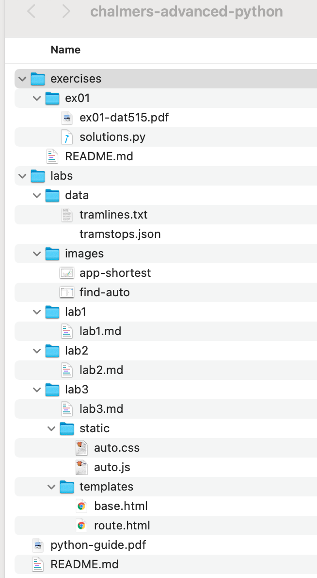
Our simple JSON encoding represents
- each directory name as a key with a subtree as value,
- each file name as a key with null as value.
Then the exercises subdirectory is represented as
{
    "chalmers-advanced-python": {
        "exercises": {
            "ex01": {
                "ex01-dat515.pdf": null,
                "solutions.py": null
            },
            "README.md": null
        }
    }
}
Constructing the tree for the whole directory in the picture is left as an exercise. The best way to do this is to automate it by writing a function which, for any directory, constructs a dictionary from which the JSON object can be dumped, by using
os.listdir(dir)to list the contents of a directory,os.path.isdir(file)to test if a file is a directory,os.path.join(path, file)to add a path to a file name.
from the Operating System library os (https://docs.python.org/3/library/os.html).
Trees are also a special case of graphs, which will have a central role in Labs 2 and 3.
5. Graphs and graph algorithms
We will cover most of the material that will be needed for the first part of Lab 2. We will illustrate the presentation with the tram network graph built in Lab 1, but also with other graphs - mostly smaller, but also some that are much larger.
5.1. What is a graph
We will start with the usual definition of graphs in discrete mathematics and computer science, as explained for instance on Wikipedia: https://en.wikipedia.org/wiki/Graph_(abstract_data_type)
A graph consists of:
- a set of vertices, also known as nodes
- a set of edges, also known as links, that connect pairs of vertices
The following picture shows a simple graph with 7 vertices and 8 edges:
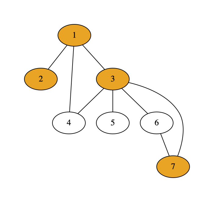
The coloured vertices mark the shortest path from vertex 2 to vertex 7. Finding shortest paths is one of the most well-known graph algorithms, used in numerous route-finding systems and also in our Lab 2. The shortest path in this simple case is the traversal that goes through the minimum number of vertices. This is why for instance the transition from 3 to 7 is by the direct edge, not via vertex 6.
The above picture shows an undirected graph, which means that transitions are possible in both directions at every edge. In a directed graph, edges are one-way streets, which in diagrams are marked with arrow heads pointing to one direction. The following graph has the same vertices and edges as before, but now directed.
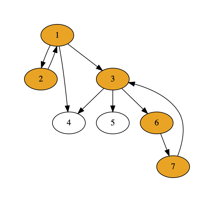
Notice that the shortest path from 2 to 7 is now different, since the direct line from 3 to 7 is no more available. Also notice that we have 2 edges connecting 1 and 2, to mark that both directions are possible.
The shortest path solution can also vary because of weights associated with edges, also known as costs. Imagine, for instance, that the direct way from 3 to 7 is with a super fast special train that costs 4 times as much as a usual ticket. If we use price as cost function, the shortest path algorithm now gives us the cheapest path. In the following picture, we have marked the prices as weights of edges. Since the price is used as cost function, the shortest path from 3 to 7 is different from the the first graph where, technically, the cost function is a constant function.
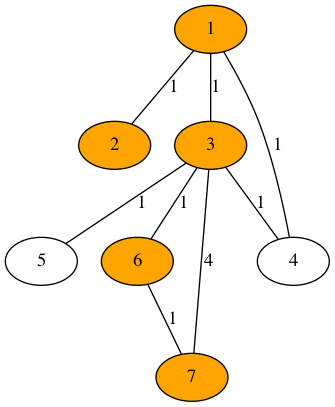
5.2. Graphs for transport networks
In Labs 2 and 3, we are will work with undirected graphs, because it is a feature of Gothenburg tram lines that they can always be traveled in both directions. However, since this is not a universal feature of transport networks, our data types and algorithms should also be ready for directed graphs. If properly designed, this generality comes with very little overhead in the code - and such design is, indeed, one of the wider learning outcomes of this course.
Weights and cost functions will, however, play an important role for us. In general, the best path in a network can depend on many different things:
- time,
- geographical distance,
- price,
- number of changes,
- preference to travel via a certain place or route,
- preference to use a certain mode of transport (tram, bus, ferry) or provider (train company, airline).
Full-scale travel planning applications can optimize for all these features, and many more. Also our solution in Lab 2 will be ready for this. But the final app in Lab 3 will only consider time, distance, and number of changes.
The following picture shows the Gothenburg tram network as a graph built from the data from Lab 1, with a shortest path from Chalmers to Komettorget.
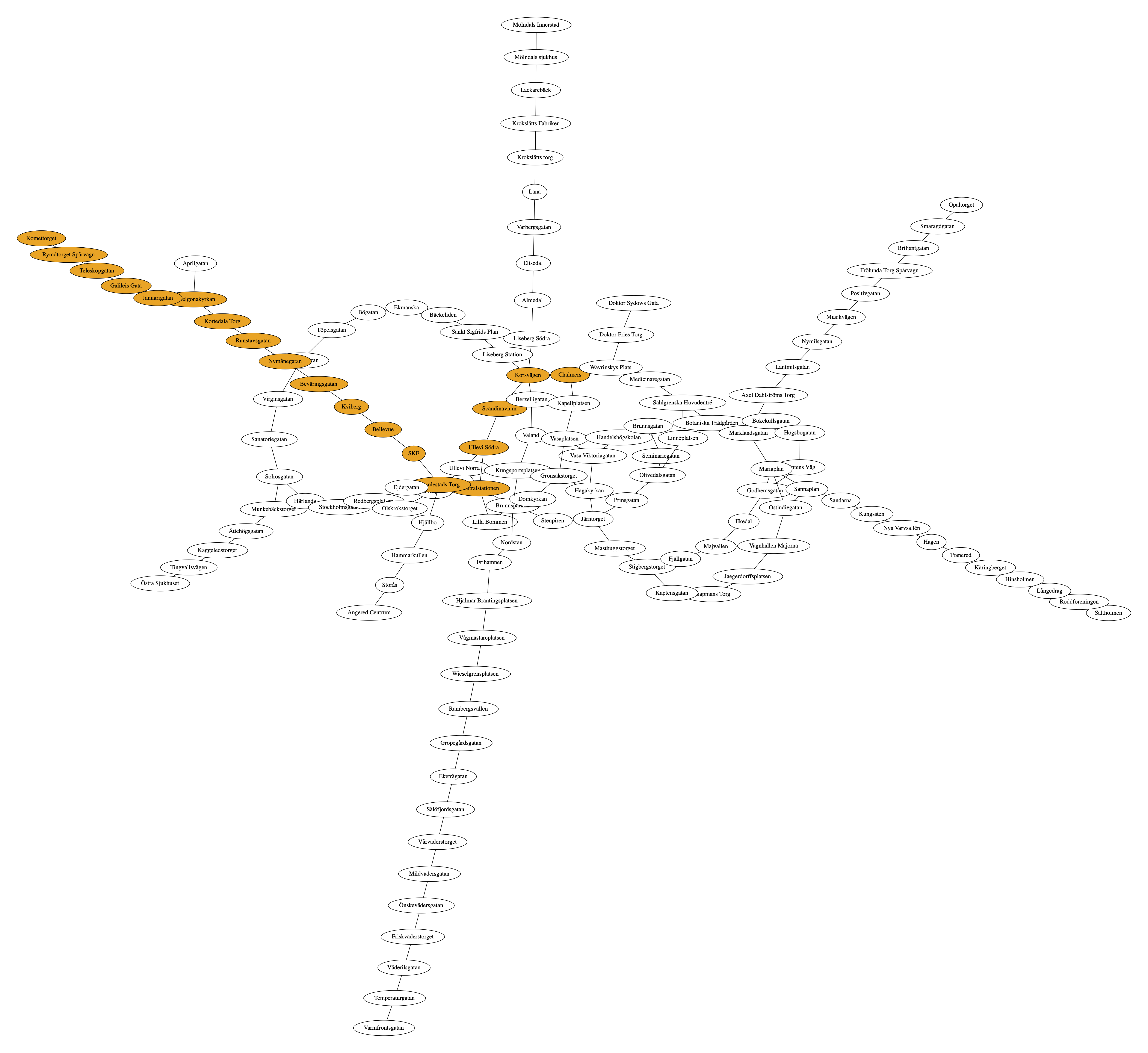
This is the level of visualization we will reach in Lab 2. In Lab 3, visualization is a central topic, and we will be able also to show
- stops in realistic geographical locations,
- colours of tram lines,
- different colours for shortest time and shortest distance, if different.
The picture at the beginning of this document is the corresponding screenshot form the app.
5.3. Representations of graphs
A graph is, mathematically, given by
- a set of vertices,
- a set of edges, represented by pairs of vertices.
The set of vertices might look redundant, since it can usually be derived from the set of edges. However, since graphs can also contain isolated vertices (with no edges), it is necessary to include that set. (If storage space is to be optimized, it is of course enough to store the isolated vertices, but this is not what we are going to do.)
In undirected graphs, edges (a, b) and (b, a) are considered equal, and need not be repeated.
In directed graphs, each of the pairs must be stored separately, if both directions work.
(Alternatively, one can save space by using a special format or separate set for bidirectional edges, but this is again something we will not consider.)
A straightforward representation of our first example graph,
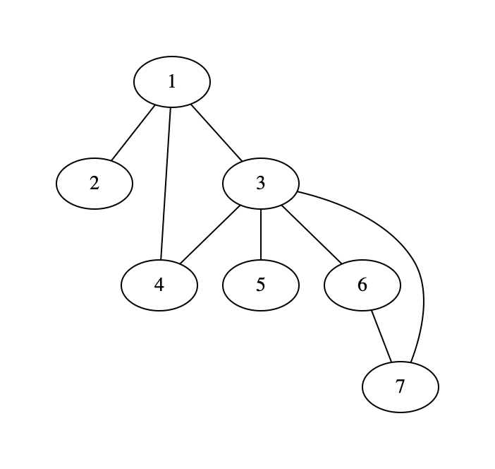
is thus with two sets - in Python notation,
vertices = {1, 2, 3, 4, 5, 6, 7}
edges = {(1,2), (1,3), (1,4), (3,4), (3,5), (3,6), (3,7), (6,7)}
An alternative to this representation is adjacency list: a dictionary which to every vertex associates the set of its neighbours - that is, the vertices to which it has an edge.
adjlist = {
    1: {2, 3, 4},
    2: {1},
    3: {1, 4, 5, 6, 7},
    4: {1, 3},
    5: {3},
    6: {3, 7},
    7: {3, 6}
}
In this representation, we do not need to store vertices separately, since isolated vertices have simply an empty list associated. Notice also that neighbours are given in both directions even for thie undirected graph. This is not necessary for data representation, and actually introduces a potentially harmful redundancy, but it makes it faster to look up the neighbours of each vertex. A possible non-redundant representation is:
adjlist = {
    1: {2, 3, 4},
    2: set(),
    3: {4, 5, 6, 7},
    4: set(),
    5: set(),
    6: {7},
    7: set()
}
where only the neighbours denoted by larger numbers are shown. To get all neighbours of a given vertex from this representation requires, in addition to a lookup with that vertex as a key, a scan of all larger vertices.
Yet another representation is adjacency matrix, which is a square matrix with rows and columns for every vertex. Every cell (i,j) has value 1 if there is an edge from i to j, otherwise 0. The simplest Python representation is a list of lists:
[
    [0, 1, 1, 1, 0, 0, 0],
    [1, 0, 0, 0, 0, 0, 0],
    [1, 0, 0, 1, 1, 1, 1],
    [1, 0, 1, 0, 0, 0, 0],
    [0, 0, 1, 0, 0, 0, 0],
    [0, 0, 1, 0, 0, 0, 1],
    [0, 0, 1, 0, 0, 1, 0]
]
together with the list of vertices, which gives the order in which the rows and columns represent the vertices.
Adjacency matrices are easy to generalize to weighted graphs: store the weight of the edge instead of 1, and None instead of 0.
They are not optimal for sparse graphs, for which they contain mostly zeros.
Therefore we will not use them in our lab, but you can consider them as an exercise.
The three representations of graphs mentioned above can be converted to each other, which will be one of the tasks in Lab 2. They also enable the most important graph operations, which are needed when graphs are used in computing tasks.
- looking up neighbours,
- looking up predecessors and successors (a subdivision of neighbours in directed graphs),
- adding and removing edges and vertices,
- getting and setting weights of edges,
- getting and setting values of vertices, which means extra information associated with them (for instance, the geographic locations of tram stops).
Now it is time to set this all in practice and look at the implementation details.
5.4. Implementing graphs in Python
This section is closely related to Lab 2 specification.
We will define a class, to be named Graph, to store graphs.
The class will have an internal storage of vertices and edges, using internal (hidden) instance variables.
As the case is in Python, we cannot really make these variables “private”, but we can give them names that start with underscores, which is a Python convention to mark this intention.
More important than naming is to make sure that the hidden variables are never needed when graphs are used, but that enough “public” methods are provided by the class.
We will go into more details about class definitions in next chapter. Here it is enough to show the shape of the expected class definition:
class Graph:
    def __init__(self, adjs=None, values = None, directed=False):
        "can initialize with an adjacency dict and a value dict"
        self._adjdict = adjs or {}
        self._valdict = values or {}
        self._isdirected = directed

    # here are some of the public methods to implement
    def vertices(self): ...
    def edges(self): ...
    def neighbours(self, v): ...
    def add_edge(self, a, b): ...
    def add_vertex(self, a): ...
    def is_directed(self): ...
    def get_vertex_value(self, v): ...
    def set_vertex_value(self, v, x): ...
We have made some design choices that could be made differently, as you will notice if you look at graph implementations in other sources:
- We choose to store the graph internally as an adjacency dictionary.
- We enable initializing the graph with an adjacency dictionary.
- We use the same class for directed and undirected graphs.
- We include the values of vertices in the basic Graph class, as a dictionary that can optionally be provided by
__init__().
Important note: we use None as the default value for both the start and values arguments.
A more natural choice would be an empty dictionary.
However, since dictionaries are mutable objects, and since the evaluation of default arguments is performed only once, changes in these objects in any instance of the Graph class would also affect all other class instances.
This is the behaviour that the official Python tutorial, section 4.8.1, warns about.
A weighted graph is a subclass, which just adds weights of edges (such as transition times between tram stops):
class WeightedGraph(Graph):

    def set_weight(self, a, b, w): ...

    def get_weight(self, a, b): ...
All of this will be your job in Lab 2 to implement.
Since this is a subclass of Graph, we will postpone the discussion on its initialization until we introduce inheritance.
5.5. The shortest path algorithm
The algorithm to be used in both Lab 2 and Lab 3 is the shortest path algorithm named after the Dutch computer scientist E.W. Dijkstra, who invented this algorithm in 1956. Therefore it is commonly known as Dijkstra’s algorithm.
If you want to make your own implementation, you can follow the pseudocode here: https://en.wikipedia.org/wiki/Dijkstra%27s_algorithm The same page also gives animations and explanations.
In Lab 2, however, you will be able to use the NetworkX library (https://networkx.org/). You just need to figure out how to apply it to your own tram network graph and how to vary the definition of “shortest”: it can be distance, it can be time, maybe even price. The algorithm is general enough to compute the best path according to any such criterion.
And much more details and depth about graph and other algorithms (including stacks and queues) can be found from data structure courses and books. The following free on-line books are used at the Chalmers course:
https://runestone.academy/runestone/books/published/pythonds3/index.html
You can also take a look at the networkx library, which is designed to work for large and complicated graphs of various kinds.
5.6. Baseline visualization
We will use the graphviz library (https://graphviz.readthedocs.io/en/stable/api.html).
Not very much will be needed at this point.
The main things are:
- the class
graphviz.Graph, - its method
node(v)to add a vertex, - its method
edge(v, w)to add an edge, - its method
render()to draw the graph.
And yes, the Graph class has the same name as our class, but this is no problem unless we import * from graphviz.
The basic algorithm in visualization is simply:
- create an instance of
graphviz.Graph, - loop over the vertices of your graph applying
node()to them, - loop over the edges of your graph applying
edge()to them, render()the result
We will come back to visualization in Chapter 7 and introduce more functionalities of graphviz but also take a look at other visualization libraries.
5.7. Other examples of graphs
5.7.1. Knowledge graphs from WikiData
WikiData is a knowledge base that is increasingly used for storing facts reported in the Wikipedia:
https://www.wikidata.org/wiki/Wikidata:Main_Page
A direct way to use WikiData is to send SPARQL queries, using the query language SPARQL (SPARQL Protocol and RDF Query Language). SPARQL has some similarities with SQL, but it is designed for graph databases rather than relational ones.
Graphs in WikiData consist of RDF triples, (Resource Description Framework), which are meant to represent the subject-predicate-object relations. Here are examples from the Swedish Royal Family:
- CarlGustaf-father-Victoria
- Silvia-mother-Victoria
Such triples can obviously be used for building graphs, where subjects and objects are vertices and predicates are labeled edges.
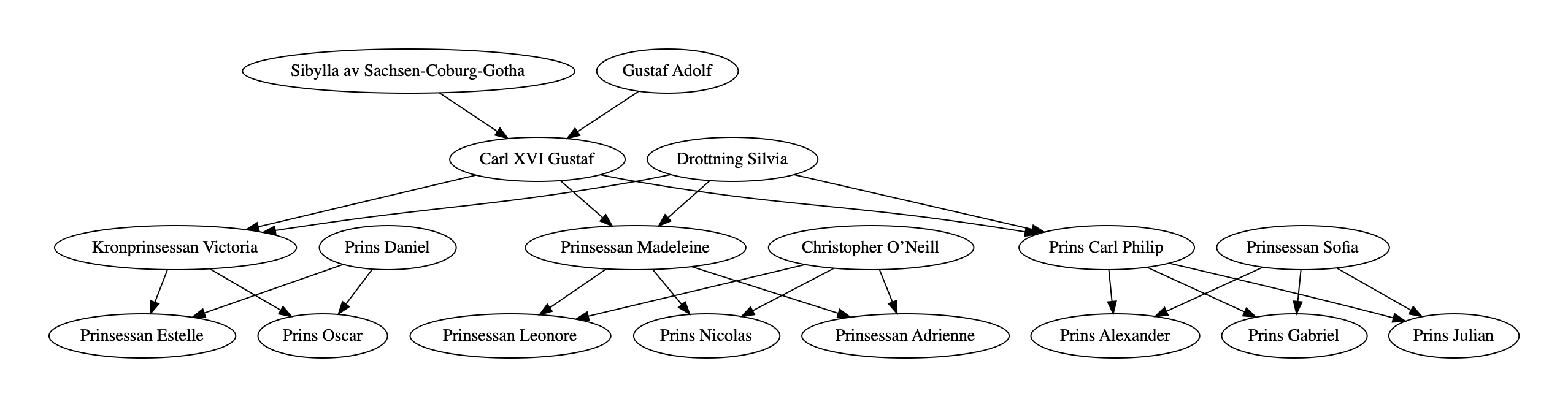
The query for retrieving this data can be found here: https://w.wiki/4BX9
A special feature of knowledge graphs is that there can be more than one edge between two vertices, representing different relations. For instance, a person can be the mother of another one, and at the same time her teacher. How to represent these situations will be left as an exercise in object-oriented design.
5.7.2. Maps and graph colouring
Another example from WikiData is built on the relation “country X is a neighbour of country Y”: https://w.wiki/4EuG
This graph can be used as input for a graph colouring algorithm, which enables always selecting different coulours for countries that are neighbours. The famous four-colour theorem. states that planar graphs - of which two-dimensional maps are an example - it are always possible to colour by just four different colours. An example is a map of Europe coloured by using the algorithm:

Deciding if a graph is planar is an interesting algorithmic task in itself.
5.7.3. Social networks
Social networks defined by “person X is connected to person Y” is a field where very large graphs can easily be found. Interesting questions about such graphs are
- how connected the graph is,
- how many connections persons have,
- what clusters there are, i.e. subgraphs of closely related vertices.
An anonymized example can be found at https://snap.stanford.edu/data/ego-Facebook.html
6. Object-oriented design
Python supports object-oriented program design by enabling the definition of classes as well as class hierarchies using inheritance, which can be multiple like in C++ but unlike Java. Classes also support polymorphism by method overriding, but one should at the same time point out that Python is intrinsically more polymorphic than many other languages because of dynamic typing.
Python does not support all aspects of object-oriented programming: in particular, information hiding is not forced by the language but depends totally on the programmer’s discipline in following certain conventions. Neither does Python force object-oriented programming like Java does, but permits a mixture of functions and classes like C++.
However, and very importantly, Python is inherently object-oriented due to its data model, which is entirely based on objects.
Even basic types such as int are actually types of objects in this data model.
This gives Python a special flavour that is rarely seen in elementary programming but exploited heavily in more advanced Python.
We will therefore start this chapter with an overview of Python’s data model and how it is accessed by programmers. After that, we will look at object-oriented concepts proper, focusing on the role of data abstraction and code reuse, which are essential in all program design. All high-level programming languages provide functions as a tool for this, but classes and inheritance are additional tools in object-oriented languages.
6.1. The data model of Python
The primary source for this section is Chapter 3 of the Python reference manual: https://docs.python.org/3/reference/datamodel.html Just like when reading the Tutorial, we will go through the standard document itself and just list here some highlights to which special attention should be paid.
6.1.1. Expressions, objects, and values
One central principle is the tree-partite structure:
expression - object - value
A more traditional view of programming language semantics includes just two levels: expressions and their values. Objects are then a special kind of values, other kinds being integers and floats. But in Python, all expressions primarily refer to objects, which in turn have values.
The “value of an expression” is in fact the value of the object that the expression denotes. The denotation of an expression can change, for instance, when a variable is assigned a new object. The object itself can also change, if it is mutable. Here is a minimal example:
# assign an object to x
>>> x = 7

# assign a different object to x
>>> x = [1, 2, 3]

# change the value of the object assigned to x
>>> x.append(4)
6.1.2. Types
Another special feature of Python is that objects have types but expressions do not. In Java, for instance, both expressions and objects have types, although in slightly different type systems. The “type of an expression” is the type of the object that the expression denotes at a given point of execution, and it can change. However, the type of an object does not change, according to what types mean in Python.
The concept of types itself is different from many other languages. If we do
x = [1]
x[0] = 'one'
the object denoted by x has the type list, and this does not change.
In Java and many other languages, the type would be list of integers for [0] and list of strings for ['one'].
But the types of Python are less fine-grained: lists are just lists, and they can also contain elements of many different types.
6.1.3. Mutability and other properties
One of the most important concepts concerning types is mutability. We have already seen that this is a difference between lists and dictionaries (mutable) and strings and tuples (immutable). However, the distinction (intentionally) “leaks” because even immutable types objects can contain mutable elements. If a tuple has a list as an element, the value of the tuple will change when the list element changes.
>>> xs = [1, 2]
>>> t = (xs, 3)
>>> t
([1, 2], 3)
>>> xs.append(4)
>>> t
([1, 2, 4], 3)
Mutability is one of the aspects that is reflected in error messages. For instance,
>>> x = (1, 2)
>>> x[0] = 'one'
TypeError: 'tuple' object does not support item assignment

>>> x.append(3)
AttributeError: 'tuple' object has no attribute 'append'

>>> x.sort()
AttributeError: 'tuple' object has no attribute 'sort'
At the same time, some other operations, which you might not even expect, are available:
>>> x + (3, 4)
(1, 2, 3, 4)
All of this is hidden in the normal syntax of Python, but it is not magic: it is defined via a large set of special methods, which can be provided by the programmer as a part of the definition of classes.
6.1.4. Operator overloading
Special method names are explained in Section 3.3 of the reference manual. They make it possible to define standard operations, such as arithmetic, comparison, element assignment, and iteration, for any class. This is known as operator overloading.
The special names have the format where a double underscore __ appears on both sides.
These methods are therefore sometimes called dunder methods (“double under”).
In the normal usage of classes, the programmer never sees them, but only their effects on standard Python operators such as == and +.
For many Python programmers, defining dunder methods is seldom a relevant task.
The only exception is __init__(), which defines how new instances of a class are built.
But dunder methods definitely belong to the toolbox of advanced programmers, and knowing about them gives a deeper understanding of how Python works.
Again with the official reference, Section 3.3, as our main source, the code below lists some examples of dunder methods and what their effects could be for graphs.
# __init__(), initialization:
>>> G = Graph([(1, 2), (1, 3), (2, 4)])

# __repr__(), exact representation string:
>>> print(G.__repr__())
Graph({1: [2, 3], 2: [1, 4], 3: [1], 4: [2]})

# __str__(), nice-to-read string:
>>> print(G)
{1: [2, 3], 2: [1, 4], 3: [1], 4: [2]}

# __eq__(H), equality:
>>> H = Graph([(3, 1), (4, 2), (1, 2)])
>>> print(G == H)
True

# __len__(), length:
>>> print(len(G))
4

# __getitem__(), get item by key:
>>> print(G[1])
[2, 3]

# __setitem__(), set value of key:
>>> G[1] = [4, 5]
>>> print(G)
{2: [4], 3: [], 4: [2, 1], 1: [4, 5], 5: [1]}

# __iter__(), iterate over elements:
>>> for v in G: print(G[v])
[4]
[]
[2, 1]
[4, 5]
[1]

# __add__(H), addition:
>>> print(G + H)
{2: [4, 1], 4: [2, 1], 1: [4, 5, 3, 2], 5: [1], 3: [1]}

# __neg__(), unary negation:
>>> G = Graph([(1, 2), (1, 3), (2, 4)], directed=True)
>>> print((-G).edges())
[(2, 1), (3, 1), (4, 2)]
>>> print(-G == G)
False
Some examples of special “dunder” methods as defined for graphs.
The definitions of these methods is not always obvious. If there is no natural choice, it is usually better not to define them. Let us consider just one example: unary negation:
def __neg__(self):
    if self.is_directed():
        H = Graph(directed=True)
        for (a, b) in self.edges():
            H.add_edge(b, a)
        return H
    else:
        raise TypeError('bad operand for unary .: undirected graph')
The idea is that only directed graphs can be negated, by reversing all the edges.
For undirected graphs, a TypeError is raised, similar to what you get when for instance trying to negate a string or a list.
This definition of __neg__() does make some sense, but it is by no means obvious.
It could be compared to defining the negation of a list as its reverse.
Since this is not provided by standard Python, we would actually rather not define negation for graphs either.
6.2. How to define classes
Python’s class definitions have an extremely liberal format: they can consist of any block of statements. However, there is a standard format that we want to encourage, which comes close to the more disciplined way of defining classes in languages like Java and C++. The format is shown below:
class C(B):
    """
    doc string explaining what the class is about
    """

    def __init__(self, ...):
        """
        doc string explaining what the arguments mean
        and what happens when an instance is created
        """

        # running the init of base class B, if any
        super().__init__(...)
        ...
        # setting initial values of instance variables
        self._x = ...
        self._y = ...

    # public getter and setter methods, possibly with doc strings
    def get_x(self)
    def set_x(self, v)

    # dunder methods, if any
    def __eq__(self, other)

    # other public methods
    ...
The components of a disciplined definition of a class. A concrete example is given below:
class Graph:
    """
    A class of undirected graphs.
    """
    def __init__(self):
        """Start with an empty graph."""
        self._adjlist = {}

    def add_edge(self, a, b):
        """Add an edge, and the vertices if needed."""
        if a not in self._adjlist:
            self._adjlist[a] = set()
        self._adjlist[a].add(b)
        if b not in self._adjlist:
            self._adjlist[b] = set()
        self._adjlist[b].add(a)

    def vertices(self):
        """Lists all vertices."""
        return self._adjlist.keys()

    def edges(self):
        """Lists all edges in one direction, a <= b"""
        eds = []
        for a in self._adjlist.keys():
            for b in self._adjlist[a]:
                if a <= b:
                    eds.append((a, b))
        return eds

    def __str__(self):
        """Shows the adjacency list."""
        return str(self._adjlist)

    def __getitem__(self, v):
        """Gives the neighbours of vertex v."""
        return self._adjlist[v]
A minimal class for graphs, showing examples of “private” variables (_adjlist),
invariant enforcement (add_edge()),
and “dunder” methods (__init__(), __str__(), __getitem__()).
6.3. Abstraction
One of the most important goals of object-oriented design is data abstraction. The user of a class (i.e. other classes and functions referring to it) should neither be able nor have a need to access the internal structure of the data. Instead, they should only manipulate it via getter and setter methods.
6.3.1. Building for future improvements
In the Graph class, the internal structure is the adjacency list.
This structure could quite as well be a matrix or something else;
it could even be delegated to some other class whose internals are in turn unknown to us, for instance the Graph class of the networkx library: this is one possible way to solve Lab 2.
When our program is developed further, we can silently change the internal representation without causing any harm to the users.
For example, we could switch to an ultra-efficient matrix representation from the numpy library if our graphs grow beyond the limits that we had first imagined.
Such changes often happen when new, improved versions of software libraries are released.
Data abstraction guarantees that they do not break the code written by users of the libraries: on the contrary, their code can be improved for free thanks to improvements in libraries.
6.3.2. Invariants
Another reason for data abstraction is that it can enforce invariants, properties that the data should satisfy at all times. In the undirected graph, the invariant is that, whenever a a is a neighbour of b, then also b is a neighbour of a. If the internal representation is adjacency lists represented by dictionaries, we have
invariant: if a in _adjlist[b] then b in _adjlist[a]
If the user of the Graph class changes _adjlist directly, there is a risk that the invariant gets violated.
Therefore, the user should only use the public methods, where
-
add_edge(a,b)adds to both_adjlist[b]and_adjlist[b] -
remove_edge(a,b)removes from both_adjlist[b]and_adjlist[b]
Maintaining invariants like this is, as a general rule, the responsibility of the author of the class, not of its user.
6.4. API
One good way to achieve data abstraction is to keep the instance variables hidden from users.
We must then make sure that all possible operations that we want the users to be able to do are doable by the public methods.
To make the distinction clear, we can use underscored names to mark private variables and methods.
This is, of course, a much weaker protection than the private, protected, and public keywords in Java and C++, which are checked to be obeyed at compile time.
The public methods of a class form its API, Application Programming Interface.
The __init__() method is a part of the API, although not by this name, but by using the class name, which is known as the constructor of the class:
C.__init__(self, args) is documented as C(args) in the API.
For Python programs, documentation can be automatically generated with the pydoc program (which may be named pydoc3 in your system):
$ pydoc3 -w trees
wrote trees.html
In addition to the help() function, this is the place where document strings are shown.
The following picture shows a part of the documentation generated by this command.
The documentation hides, by default, the instance variables and only shows the methods.
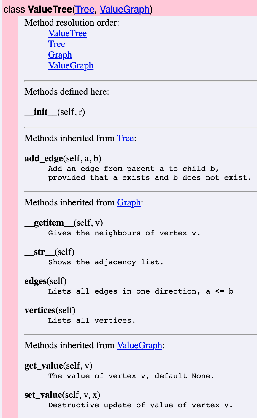
This example shows at the same time how names are resolved with multiple inheritance.
6.5. Non-redundancy and the DRY principle
Redundancy, “saying the same thing twice”, is in general a bad thing in both data representation and algorithms. This is commonly known as the DRY principle:
DRY: Don’t Repeat Yourself.
An example is, when in Lab 1 and also in Lab 2, we store the transition time from A to B in only one place - for instance, in timedict[A] if A is alphabetically before B.
In this way, we can save space but also guarantee the invariant that the time from A to B is always the same as from B to A.
The function or method for looking up transition times should then be aware of this rule and not fail when A is not covered by timedict[B].
But we have also seen a counterexample to DRY: storing each graph edge (a,b) in the adjacency list of both a and b. The reason behind this decision is that we want to look up all neighbour of any vertex efficiently. If the edge were only stored for a, we would in the worst case need to go through the whole adjacency list to find the neighbours of b. This intentional introduction of redundancy violates the DRY principle and comes with a real risk of inconsistency.
However, the risk of inconsistency is mitigated by data abstraction: the user of the class, when adding an edge to the graph, only needs to write add_edge(a, b), and the internal dictinary is updated in both direction.
Hence, in a sense, the DRY principle continues to hold for the user of the class, who does not need to add edges in both directions.
It also holds for the author of the class, in the sense that the repetition is uniformly created in one single place, the definition of add_edge().
Another use of the DRY principle is in program code. Beginning programmers, or the ones we called occasional programmers in Section 1.2.3, often program by “copy and paste”, repeating chunks of code in different places of the program. This implies a similar risk of inconsistency as the redundancies in data storage: you make a change (such as fixing a bug) in one place where the code appears, but not in all other places.
The primary way to avoid code repetition, in any high-level programming language, is functions:
Whenever you find yourself programming by copy and paste, write a function instead.
Object-oriented languages, like Python, add to this the concept of classes and inheritance:
Whenever a class shares some properties of another class, consider implementing it as a subclass.
6.6. Inheritance
In the lecture, we go through an example in live coding, defining
- the class
ValueGraphas subclass ofGraph, - the class
Treeas subclass ofGraph, - the class
ValueTreeas subclass of bothValueGraphandTree.
The resulting code is shown below:
class ValueGraph(Graph):
    """Graph where vertices have values."""
    def __init__(self):
        """Initialize with empty graph and no values."""
        super().__init__()
        self._valuelist = {}

    def get_value(self, v):
        """The value of vertex v, default None."""
        return self._valuelist.get(v, None)

    def set_value(self, v, x):
        """Destructive update of value of vertex v."""
        if v in self.vertices():
            self._valuelist[v] = x


class Tree(Graph):
    """Trees as graphs with certain restrictions."""
    def __init__(self, r):
        """Initialize with a root node r."""
        super().__init__()
        self._adjlist = {r: set()}

    def add_edge(self, a, b):
        """
        Add an edge from parent a to child b,
        provided that a exists and b does not exist.
        """
        if a not in self._adjlist:
            print('Parent does not exist:', a)
        elif b in self._adjlist:
            print('Child already exists:', b)
        else:
            self._adjlist[a].add(b)
            self._adjlist[b] = set()


class ValueTree(Tree, ValueGraph):
    def __init__(self, r):
        super().__init__(r)
Notice, in particular, that
- a
Treemust have at least one node, the “root”; add_edge()inTreeis quite different fromGraph, since in a tree, each node (must have exactly one “parent”, except the root, which has no parents.
Trees are in many ways a subclass of graphs, and defining them in this way makes many graph algorithms (such as search and visualization) available. However, in some other contexts it could be better to define tree as a class of its own, constructed recursively from a root and its subtrees. The construction of a graph could then be a function or method of trees.
6.6.1. Diamond problems
The three classes form a hierarchy, which moreover shows multiple inheritance and therefore has the shape of a diamond, which is clearly seen in the diagram in the UML diagram below.
This gives rise to diamond problems, where the same method or variable could be inherited from different superclasses.
In our case, the method add_edge() is defined in both Tree (overriding Graph) and ValueGraph (just inheriting it from Graph).
The solution of diamond problems in Python is covered by a long discussion in:
https://www.python.org/download/releases/2.3/mro/
In a simple case like ours, the resolution order is depth-first, left to right, as
shown in the generated documentation above.
The general MRO (Method Resolution Order) algorithm is more complicated.
The special variable __mro__ provides the way to inspect the method resolution order of a class:
>>> ValueTree.__mro__
(<class 'trees.ValueTree'>, <class 'trees.Tree'>, <class 'trees.ValueGraph'>, <class 'trees.Graph'>, <class 'object'>)
(the class object is implicitly a base class of all classes in Python).
If we had written the inherited modules in the opposite order:
class ValueTree(ValueGraph, Tree)
the result would have been different - and not what we wanted.
We could of course even then restore intended add_edge() method by overriding the one in ValueGraph, but this would not be maximal reuse of code.
Intuitively, ValueTree has “more in common” with Tree than with ValueGraph, which explains the order we chose.
But this is not always clear, and some object-oriented languages - in particular, Java - have chosen not to permit multiple inheritance at all.
6.7. UML, Unified Modelling Language
UML, Unified Modelling Language is a graphical notation for visualizing classes and their relations.
The image below shows an example of a UML diagram representing the classes defined in trees.py.
Each box represents a class, divided into three sections: the class name, instance variables, and methods.
Triangle-headed arrows mark inheritance.
Inherited variables and methods are marked only if the subclass overrides them.
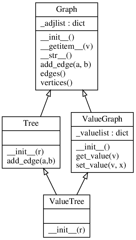
The diagram is slightly edited from one obtained automatically with a tool, documented in https://gist.github.com/HarshaVardhanBabu/9a47db9e33cf06e9e1e917520bb54056.
The tool was applied to my Lab 2 solution with the commands:
$ pyreverse --filter-mode=ALL trees.py
$ dot -Tpng trees.dot > trees.png
The latter command uses GraphViz to generate the actual visualization.
This way of using UML, after the implementation, serves the purpose of documentation. A more widely recommended use is before the implementation, for the design of classes. However, a strictly linear first-design-then-implement workflow is not always the most productive way to program. It can be more natural to jump back and forth between code and a higher-level design view. In this use, UML can be a good tool, since it shows at a glance if there is something strange in the implementation, which can then be corrected and a new UML generated.
7. Testing
Testing implies verifying a piece of code (or part of it) for its behavior—be it functional, non-functional, or quality behavior. One obvious way of testing one’s code is to run it several times with various inputs—often testing boundary conditions, equivalence classes etc.—and observe the output. This form of testing requires the tester to correctly identify input scenarios in which a code can behave erroneously. However, this form of manual testing is laborious, and one may not be able to imagine and test every possible scenario. Python provides several methods to test code’s behavior. In the following, we discuss some of the most common methods.
7.1. Manual testing
The simplest form of testing involves repeatedly running the code with varying inputs to test if code behaves as expected. For example, consider the following graph storage format converter. One way to test if it works correctly is by repeatedly executing the file with various inputs and note the behavior.
def graph_convert(graph):
    '''
    This functions converts a graph to an alternative format. If the input is
    an adjencecy matrix (2-D list), it converts it to an adjencecy dictionary.
    If the input is an adjencecy dictionary, it is converted to an adjencecy
    matrix. The result is returned to the caller.
    '''

    if isinstance(graph, dict):
        # if input graph is dict:
        adj_mat = [
            [
                1 if j in graph.get(i, []) else 0
                for j in range(len(graph))
            ]
            for i in range(len(graph))
        ]
        return adj_mat

    elif isinstance(graph, list):
        # if input graph is matrix:
        adj_dict = {
            row_no: [ j for j in range(len(graph))
                     if graph[row_no][j] ]
            for row_no in range(len(graph))
        }
        return adj_dict

    else:
        # the input is not in expected format
        return None
However, to test it systematically, we need to use some testing framework.
7.2. Testing frameworks in Python
A testing framework in python refers to a systematic way of automating code testing. It is typically provided by libraries or modules, some of which are already built-in in python. A few popular examples include unittest (built-in), pytest, and hypothesis.
7.3. The unittest library
To test the graph_converter function, we develop a test case with unittest library in this section. A test case is a class with testing code which inherits from unittest.TestCase base class provided by the unittest framework. A test case class contains some test methods which test the code by calling appropriate functions, creating objects, and assert-ing some expressions. A test suite aggregates one or more test classes, and test methods to form a meaningful testing group.
To test the graph_converter we write TestGraphConvert test case. This class is saved in test_graph.py which resides in the same project directory. The test case class contains a test method test_dict2mat. Please note the naming conventions here. The class, the methods, and the file all start with test prefix. It is customary and facilitates automation of test case collection/execution by the test runner.
# file: test_graph.py
import unittest
import graph_converter as gc

class TestGraphConvert(unittest.TestCase):
    '''This class tests the behaior of graph convertor function.'''
    def test_dict2mat(self):
        '''This methods tests dictionary to matrix conversion'''
        self.adj_dict = {0: [1, 2], 1: [0, 2], 2: [1, 0, 3], 3: [2]}
        self.expected = [[0, 1, 1, 0], [1, 0, 1, 0], [1, 1, 0, 1], [0, 0, 1, 0]]

        self.returned_mat = gc.graph_convert(self.adj_dict)

        self.assertIsInstance(self.returned_mat, list,
                        f'Returned output is not a matrix')
        self.assertEqual(self.returned_mat, self.expected,
                         f'Returned matrix is not as expected: {self.expected}')
The test_graph.py imports unittest and the graph_converter which it needs to test. We then write a simple test method test_dict2mat. This test method calls our target function graph_convert and passes an adjacency dictionary self.adj_dict. We also create self.expected to store what we expect as the result of our function call. Once graph_convert returns a value, we assert two tests. First, we check if the returned value has <list> as type. Second, we assert that the returned value should match what we expect. The message in assert statements is displayed if an assertion fails.
The unittest has its own pool of assertion methods which you shall read about in the official documentation. A typical assert method call is of the form
<assert_method>(<recieved data to test>, <expected data to match>, <message (optional) to display if the test fails>)
The test cases can run in several ways. We recommend that you initially run it with verbose switch -v which brings more information, though You can run your testsuite without it. The output from our test run shows that the test_dict2mat test method passed. The output also shows how much time was consumed.
$ python3 -m unittest -v
test_dict2mat (test_graph.TestGraphConvert.test_dict2mat) ... ok

----------------------------------------------------------------------
Ran 1 test in 0.000s

OK
Expanding the previous example, we now want to test the functionality for converting an adjacency matrix to an adjacency dictionary, and also want to test if graph_convert behaves as expected on invalid parameters. These behaviors are tested by test methods test_mat2dict and test_invalid_input respectively.
# file: test_graph.py
import unittest
import graph_converter as gc

class TestGraphConvert(unittest.TestCase):
    '''This class tests the behaior of graph convertor function.'''
    def test_dict2mat(self):
        '''This methods tests dictionary to matrix conversion'''
        self.adj_dict = {0: [1, 2], 1: [0, 2], 2: [1, 0, 3], 3: [2]}
        self.expected = [[0, 1, 1, 0], [1, 0, 1, 0], [1, 1, 0, 1], [0, 0, 1, 0]]

        self.returned_mat = gc.graph_convert(self.adj_dict)

        self.assertIsInstance(self.returned_mat, list,
                        f'Returned output is not a matrix')
        self.assertEqual(self.returned_mat, self.expected,
                         f'Returned matrix is not as expected: {self.expected}')

    def test_mat2dict(self):
        '''This methods tests matrix to dictionary conversion'''
        self.adj_mat = [[0, 1, 1, 0], [1, 0, 1, 0], [1, 1, 0, 1], [0, 0, 1, 0]]
        self.expected = {0: [1, 2], 1: [0, 2], 2: [1, 0, 3], 3: [2]}

        self.returned_dict = gc.graph_convert(self.adj_mat)

        self.assertIsInstance(self.returned_dict, dict,
                        f'Returned output is not a dictionary')
        self.assertEqual(self.returned_dict, self.expected,
                         f'Returned dictionary is not as expected: {self.expected}')

    def test_invalid_input(self):
        '''This methods tests if converter function returns None with invalid input'''
        self.input = 'something else than a matrix of a dictionary'
        self.expected = None

        self.returned_val = gc.graph_convert(self.input)

        self.assertIsNone(self.returned_val, "Expected None, but recieved something")

if __name__=='__main__':
    unittest.main()
The unittest.main provides entry point to the unittest framework. When this function is called, it scans all your classes inherited from the unittest.TestCase superclass. It then goes on to find all methods in all such classes which have a test prefix in their names. All those methods are then executed in alphabetical order.
$ python3 -m unittest -v
test_dict2mat (test_graph.TestGraphConvert.test_dict2mat)
This methods tests dictionary to matrix conversion ... ok
test_invalid_input (test_graph.TestGraphConvert.test_invalid_input)
This methods tests if converter function returns None with invalid input ... ok
test_mat2dict (test_graph.TestGraphConvert.test_mat2dict)
This methods tests matrix to dictionary conversion ... FAIL

======================================================================
FAIL: test_mat2dict (test_graph.TestGraphConvert.test_mat2dict)
This methods tests matrix to dictionary conversion
----------------------------------------------------------------------
Traceback (most recent call last):
  File "D:\Code\DAT690\DAT690-Practice\graphs\test_graph.py", line 28, in test_mat2dict
    self.assertEqual(self.returned_dict, self.expected,
    ~~~~~~~~~~~~~~~~^^^^^^^^^^^^^^^^^^^^^^^^^^^^^^^^^^^
                     f'Returned dictionary is not as expected: {self.expected}')
                     ^^^^^^^^^^^^^^^^^^^^^^^^^^^^^^^^^^^^^^^^^^^^^^^^^^^^^^^^^^^
AssertionError: {0: [1, 2], 1: [0, 2], 2: [0, 1, 3], 3: [2]} != {0: [1, 2], 1: [0, 2], 2: [1, 0, 3], 3: [2]}
- {0: [1, 2], 1: [0, 2], 2: [0, 1, 3], 3: [2]}
?                              ---

+ {0: [1, 2], 1: [0, 2], 2: [1, 0, 3], 3: [2]}
?                            +++
 : Returned dictionary is not as expected: {0: [1, 2], 1: [0, 2], 2: [1, 0, 3], 3: [2]}

----------------------------------------------------------------------
Ran 3 tests in 0.001s

FAILED (failures=1)
Note that the failure occurs in test_mat2dict method, where the returned dictionary does not match with our expected dictionary. If you look closely, the problem arises in the following part of returned dictionary:
… 2: [0, 1, 3] …
while expected dictionary is as below:
… 2: [1, 0, 3] …
This difference of order in the list may not be significant in the context of a graph. That means, in a graph’s syntactical sense, these values mean the same edges between same vertices. However, in a pythonic context they are different due to lists being ordered structures. Therefore, you should be careful about such situations.
Interpreting the output
A ‘ . ’ in the test output indicates a passed test. An ‘ F ’ appears for a failed test. The failed test also shows further information about cause of the failure, as well as displays the message which programmer has provided in the test case. Sometimes, you may see an ‘ E ’ which means the test method has encountered an error. The error message is typically verbose.
Some good things to know
If you need to test the behavior of a class, you need to import that class in your test file and make its object for testing. You can make this test object separately for each test method, or you can make one object in setUp method which can then be used by several test methods, as shown in the example code below.
import unittest
from calc import Calc

class TestDiff(unittest.TestCase):
    '''test case for testing our simple calculator class.'''

    def setUp(self):
        self.testObj = Calc(55, 25)

    def test_sum(self):
        self.assertEqual(self.testObj.get_sum(), 80, "incorrect addition result")

    def test_dif(self):
        self.assertEqual(self.testObj.get_difference(), 30, "incorrect subtraction result")
Each approach has its own merits. For example, when test methods work with their own objects, they work independently of each other. One test methods does not affect another test method’s execution. On the other hand, one shared object made in setUp saves memory, and may be useful in situations where multiple behaviors successively depend upon each other. The setUp and tearDown methods in a test case are used to setup the testing environment, and clean it up after the test, respectively.
The difference between assert and <assert methods>
Python provides a builtin ‘assert’ keyword which is used to ascertain if a condition is true. If the condition becomes false, it raises an <AssertionError>
def add_integers(x, y):
    return x + y
assert add_integers(10, 15) == 5
$ python3 .\assert.py
Traceback (most recent call last):
  File ".\assert.py", line 2, in <module>
    assert add_integers(10, 15) == 5
           ^^^^^^^^^^^^^^^^^^^^^^^^^
AssertionError
The assert keyword is quite helpful for testing and debugging. However, testing frameworks have implemented their own versions of assertions, typically in form of asseertion methods. The unittest assertion methods are one such example, two of which you have seen in previous examples, namely self.assertEqual and self.assertIsNone. For a more detailed range of unittest assert methods, refer to unittest library official documentation
7.4. Property-based testing
In the previous example, where we tested the behavior of graph_convert on invalid input, you might have identified that the test case coverage was minimal. It only checked one type of invalid input, for example a <str>. However, there is a wide range of other invalid inputs which we have not yet tested, for example integers, lists, or malformed dictionaries.
Similarly, we have checked valid inputs via test_mat2dict and test_dict2mat. But we are not certain if our code works on all different kinds of valid inputs, for example, on a null graph (fully disconnected graph with no edges between vertices).
Writing test cases for an all-encompassing test input range, or for a wider coverage of scenarios, is tiresome; or not possible at all. In such situations, property-based testing proves to be useful. Property-based testing is based on Fuzzing idea, which means randomly generating large amounts of test data with the help of software. These test data often include boundary cases, invalid inputs, as well as valid inputs.
7.4.1. The hypothesis library
We have just discovered that it is significantly difficult for programmers/testers:
- to generate a large number of valid input data values
- to identify all possible invalid input classes, and to generate all possible invalid input data instances
Even if such inputs have been generated, it is difficult to automate the function/method call with this large array of inputs. To test our programs in such conditions, Python provides property-based testing, which is made available by the hypothesis library:
- https://hypothesis.works/ (main page)
- https://hypothesis.readthedocs.io/ (documentation)
The hypothesis library solves this problem with two simple mechanisms, namely given and strategies.
strategies: generates a range of random data based on some predefined strategy. A few noteable strategies include generating integers, floats, text, lists, matrices, and dictionaries.@given: in simple terms, it passes (gives) randomly generated data (by strategies) to the function we need to test and calls it repetedly until all random data instances are passed. Pythonically, this mechanism is implemented with<decorators>. The<decorators>transform (enhance) the behavior of a function. In this casegivendecorator enhances the behavior of target function in a way that it is called over and over again with the strategy-generated random input.
7.4.2. Decorators
A decorator in Python is a “function returning another function”, as explained in: https://docs.python.org/3/glossary.html#term-decorator
A decorator wraps another function (target/decorated function) inside it. It is prefixed with the @ symbol, and is written on the line before the definition of the decorated function. When the target function is called, the decorator enhances the target function’s execution by some pre-defined procedure. For an example, we define a simple print_random_no function which takes one positional argument and prints it on screen.
from hypothesis import given, strategies

@given(strategies.integers())       # the given decorator, with random integers as strategies
def print_random_no(x):             # print_random_no() defined as taking one positional argument
    print(x)

print_random_no()                   # print_random_no() called without an argument
Note that this function has no looping behvior of any sort, and also that calling this type of function typically requires passing it one positional argument. However, the output in the following shows that the function call with an argument fails with an error.
>>> print_random_no(15)
Traceback (most recent call last):
  File "<stdin>", line 1, in <module>
    import platform
TypeError: accept.<locals>.print_random_no() takes 0 positional arguments but 1 was given
The reason behind this error is the @given decorator, which sits above the decorated print_random_no function and wraps this function. Any function call to print_random_no shall now pass through @given first, which refuses to take any argument. Hence, Python refuses to take an argument in this function call.
Unintuitively, calling print_random_no without an argument results in the function being called and printing random integers over and over again.
>>> print_random_no()
0
36
-3816
25707
-4217659391690624265
-160176465046531079324348666701844897014
.
.
.
23063
-1566877652
>>>
Summarizing the above example, when print_random_no is called, @given takes over and uses strategies of integers to generate a large number of random integers. Each of the randomly generated integer is then used as an argument to call the decorated (wrapped) print_random_no function. Since there are many randomly generated integers, hence the target function is successively called multiple times (evident from the output above)
Some good things to know
The decorators have a broad use in Python beyond hypothesis testing. some popular built-in examples include @staticmethod, @classmethod and @property, commonly used to decorate classes into a better objected-oriented way. For example, @property decorator is the pythonic way of implementing access control to data. For an example, consider adding graph type property in our Graph class, as following:
class Graph:
    def __init__(self, edges=None):
        # ... other code lines to define graph
        self._type = 'undirected'   # note the underscore as the first letter, implying a private attribute

    @property
    def type(self):                 # note property type does not have a leading underscore
        return self._type

G = Graph()
print('Graph is:', G.type)         # though Graph object has no attribute named 'type'
Though the graph class does not define any attribute named type (the attribute name is _type), still the code runs successfully.
$ python3 graph.py
Graph is: undirected
The property decorator creates a (decorated) getter function which allows the property to be used as an attribute. Note that the private data member _type can still be accessed directly. Python does not have an access modifier mechanism. However, it is the pythonic way of indicating other programmers that these underscore data members are private and must be accessed (read/write) through property functions.
ALLOWED_TYPES = ['undirected', 'directed', 'undirected weighted', 'directed weighted']
class Graph:
    def __init__(self, edges=None):
        # ... other code lines to define graph edges
        self._type = 'undirected'   # note the underscore as the first letter

    @property
    def type(self):                 # note property type does not have a leading underscore
        return self._type

    @type.setter                    # note the setter name starts with property name
    def type(self, t):
        if t in ALLOWED_TYPES:      # check if input is valid
            self._type = t
        else:
            raise TypeError

G = Graph()
print('Graph is:', G.type)          # The default type is undirected
G.type = 'directed weighted'        # change graph type with setter
print('Graph is:', G.type)
The @<property_name>.setter decorator decorates the setter method. Please note that the name of this decorator should start with property name. The benefits of using this mechanism is, amongst others, to validate the input which is being set as the new value. The output is as following:
$ python3 graph.py
Graph is: undirected
Graph is: directed weighted
Similarly, the hypothesis library also has several other useful decorators. A few notable examples include:
@settings: one common use of this decorator is to modify default settings to allow more running time to time-intensive test suites.@composite: generate composite type of random data, for example lists of pairs.@example: allows programmers to supplement randomly generated data with their own examples.
Decorators are syntactic sugar
Decorators are syntactic sugar, which means that they can always be converted to “normal” syntax and thereby avoided:
@decorator
def function(...):
    ...
converts to:
def function(...):
    ...
function = decorator(function)
The decorator syntax is used when it is considered more readable, which is often the case in libraries. Hypothesis is the first example we see at this course. In our firt decorator example above, converting the decorator to normal syntax would give us:
from hypothesis import given, strategies

# @given(strategies.integers())         # The decorator is now commented out
def print_random_no(x):
    print(x)

print_random_no = given(strategies.integers()) (print_random_no)    # manual decoration
print_random_no()                       # function call, still results in multiple successive calls
Please note the braces carefully, and also note that now given does not have @ prefix now. If you are used to the decorator syntax, it will certainly look more readable! However, if you have not seen it before, it may look like magic.
The strategies in Hypothesis work as random generators, and one can save their results by the example() method.
Thus one could even avoid the use of given() by storing the generated objects in a list:
ints = []
for i in range(10):
    ints.append(st.integers().example())
You can run test functions by looping over such lists.
However, you will then miss some important functionalities that the given() function provides, so this is not the recommended way of using Hypothesis.
But trying it out in this way can help remove the magic.
7.4.3. Property-based testing: first example
Graph algorithms are very subtle, and it is easy to forget testing them with all relevant kinds of cases. Thus, it is important to test them using property-based testing. The Hypothesis documentation starts with a quick start example, which we have modified just a bit:
from hypothesis import given, strategies as st

@given(st.integers(), st.integers())
def test_ints_are_commutative(x, y):
    assert x - y == y - x

test_ints_are_commutative()
The function we want to test here is test_ints_are_commutative(x, y). It takes two integers as parameters. The statement @given(st.integers(), st.integers()) transformers the behvior of <test_ints_are_commutative>. The first strategy <st.integers()> generates random integers for <parameter x> and the second strategy <st.integers()> generates random integers for <parameter y>. The <@given> decorators makes it possible to call test_ints_are_commutative(x, y) over and over again with randomly generated input. Hence, the test case is run a large number of times with varying inputs.
When we run this (written in the file htest.py), we get:
$ python3 htest.py
    .
    .
    .
    assert x - y == y - x
           ^^^^^^^^^^^^^^
AssertionError
Falsifying example: test_ints_are_commutative(
    x=0,  # or any other generated value
    y=1,
)
The function name indicates that we wanted to test commutativity of integers (which in itself is incorrect, because commutivity is a property of operations, not of operands). However, contrary to the function name, the code indicates that we are testing commutivity of integers under subtraction operation (which obviously should fail because subtaraction operation on integers is not commutative).
Hypothesis has found the simplest possible counterexample that 0-1 is not equal to 1-0. Nonetheless, trying out the same with + instead of - has found no counterexamples because integers under addition are commutative.
Now, we are interested in more subtle properties, having to do with our own functions rather than + or - of integers.
7.4.4. Testing graph properties
A graph has several properties which needs testing. A couple of noteable examples include consistency and symmetry. Further graph properties may arise from one’s own context of graphs. For example, a typical setting may require that the graph is fully connectecd (i.e. no node has 0 degree), or self-loops are not allowed which may often be the case in a tram transport network.
Testing graph initialization and symmetry
Recall the first version of Graph class which we have created in our lecture.
class Graph:
    "This class implements an undirected graph represented by an adjacency dict."

    def __init__(self, edges=None):
        self._adjdict = {}
        if edges:
            for (a, b) in edges:
                self.add_edge(a, b)

    # setter methods
    def add_edge(self, a, b):
        "add a to the neighbours of b and vice-versa"
        self._adjdict.setdefault(a, set()).add(b)
        self._adjdict.setdefault(b, set()).add(a)

    def add_vertex(self, a):
        self._adjdict[a] = self._adjdict.get(a, set())

    def remove_vertex(self, a):
        self._adjdict[a] = set()
        for b in self._adjdict:
            self._adjdict[b].discard(a)

    # getter methods
    def vertices(self):
        return self._adjdict.keys()

    def edges(self):
        "edges in one direction"
        return {(a, b) for a, bs in self._adjdict.items()
                       for b in bs if a <= b}

    # dunder method
    def __str__(self):
        return str(self._adjdict)
First, we want to test if our graph initializes correctly with randomly generated edge data. To test this property, we generate tuples of randomly generated integers with values between 1 and 8. Please note that this choice of range is arbitrary, and respresnts that the graph will have vertices (nodes) named between 1 to 8. These randomly generated edge tuples are collected in the edge list which will be passed as an argument to our Graph class __init__ method.
Next, we define our first test method, namely test_graph_init_behavior. The @given decorator (imported as gv here) sits rights on top of our test method. Our test method recieves one instance of random data and creates a Graph object with it. The same random data is used to create expected set of edges (expect_edges) and expected set of vertices (expect_vertices). After that, we assert that this newly initialized graph shall return a set of edges and a set of vertices that match our expected sets.
Our second test method, namely test_graph_symmetry tests if the initialized graph is symmetric. This method asserts that if a graph has an edge <(a, b)>, then <a> must appear in the neighbours of <b> in graph’s adjacency dictionary, and <b> must appear in the neighbours of <a> in graph’s adjacency dictionary.
Note 1: we define our strategy again for the second test method. If we have to write more test methods, this way of defining strategy is laborious.
Note 2: one may be tempted to create one test method by putting assertions for initialization and symmetry in the same method. However, it is not recommended. We want to test different properties seprately. This shall help us in finding causes of failures easily when our test suites become large.
import unittest
from hypothesis import given as gv, strategies as st
from graphclasses import Graph

class TestGraphClassProperties(unittest.TestCase):
    "This class tests our graph class properties with hypothesis testing framework."

    @gv(st.lists(
            st.tuples(st.integers(min_value=1, max_value=8),
                      st.integers(min_value=1, max_value=8))
    ))
    def test_graph_init_behavior(self, edges):
        self.G = Graph(edges)
        expect_edges = { (min(a, b), max(a, b)) for a,b in edges}
        expect_vertices = { node for (a,b) in edges for node in (a, b)}

        self.assertSetEqual(self.G.edges(), expect_edges, 'the edges do not match')
        self.assertSetEqual(self.G.vertices(), expect_vertices, 'the nodes do not match')

    @gv(st.lists(st.tuples(st.integers(min_value=0, max_value=9),
                           st.integers(min_value=0, max_value=9))))
    def test_graph_symmetry(self, edges):
        self.G = Graph(edges)
        for a, b in edges:
            self.assertIn(a, self.G._adjdict.get(b, set()), 'a is not found in neighbours of b')
            self.assertIn(b, self.G._adjdict.get(a, set()), 'b is not found in neighbours of a')
Running our test case in verbose mode (with -v switch) produces the following output:
$ python3 test_graphclasses.py -v
test_graph_init_behavior (__main__.TestGraphClassProperties.test_graph_init_behavior) ... FAIL
test_graph_symmetry (__main__.TestGraphClassProperties.test_graph_symmetry) ... ok

======================================================================
FAIL: test_graph_init_behavior (__main__.TestGraphClassProperties.test_graph_init_behavior)
----------------------------------------------------------------------
AttributeError: 'dict_keys' object has no attribute 'difference'

During handling of the above exception, another exception occurred:

Traceback (most recent call last):
  File "D:\Code\DAT690\Lecture-testing\test_graphclasses.py", line 9, in test_graph_init_behavior
    st.tuples(st.integers(min_value=1, max_value=8),
       ^^^^^^^
  File "C:\Users\MusTafa\AppData\Local\Programs\Python\Python313\Lib\site-packages\hypothesis\core.py", line 2110, in wrapped_test
    raise the_error_hypothesis_found
  File "D:\Code\DAT690\Lecture-testing\test_graphclasses.py", line 18, in test_graph_init_behavior
    self.assertSetEqual(self.G.vertices(), expect_vertices, 'the nodes do not match')
    ~~~~~~~~~~~~~~~~~~~^^^^^^^^^^^^^^^^^^^^^^^^^^^^^^^^^^^^^^^^^^^^^^^^^^^^^^^^^^^^^^
AssertionError: first argument does not support set difference: 'dict_keys' object has no attribute 'difference'
Falsifying example: test_graph_init_behavior(
    self=<__main__.TestGraphClassProperties testMethod=test_graph_init_behavior>,
    edges=[],  # or any other generated value
)

----------------------------------------------------------------------
Ran 2 tests in 0.367s

FAILED (failures=1)
The first line of the output informs the names of test methods which were run along with their status. It is evidant that symmetry property test is passed, but the initialization behavior test is failed. The clear separation of test properties in two separate methods helps us identify the region of failure.
Further analysis of <AssertionError> reveals that the assertion self.assertSetEqual has failed because the first argument <self.G.vertices()> is of type <dict_keys>, which obviously does not support set operations, particularly set equality (tested via det difference operation here).
Note: This failure was not caught if we had used <assertEqual> instead of <assertSetEqual>. This emphasizes the importance of using appropriate assertions when testing.
Now we can refer back to our original <Graph> class and try to find the error. The first place to look is the vertices getter. Here we can see that it is returning <dict_keys>. Contrarily, we have treated our graph as a set always. Hence, we expect it to return set of vertices instead or <dict_keys>. A quick fix is to convert <dict_keys> to set before returning.
    def vertices(self):
        return set(self._adjdict.keys())
Test consistency after edge removal
In the context of Graph class from the previous section [Testing graph initialization and symmetry], we now want to test our graph for consistency after a node removal. In our previous test case class, we add another method <test_graph_consistency_after_node_removal>.
To save ourselves from writing graph initialization edge list strategy over and over again, we define it outside our test method. It can now be used for all other test methods which we write. Please note that we can also define this strategy outside of class as a function and call it in our decorator. The hypothesis library provides many more ways to define, combine, and restrict strategies, but you can get started with these simple ones to generate random graphs.
This strategy creates edge lists with minimum 5 tuples <min_size=5>, where tuples do not have self loops like (1, 1) or (2, 2) <unique_by=(lambda x: x[0], lambda x: x[1])>. We have opted this strategy because we have already tested initialization and consistency of our graph. Now we only want to test a normal sized to graph for node removal.
# example of defining strategies outside @gv decorator
nodes = st.integers(min_value=1, max_value=9)
node_tuples = st.tuples(nodes, nodes)
edge_lists = st.lists(node_tuples, min_size=5, unique_by=(lambda x: x[0], lambda x: x[1]))

@settings(deadline=None)        # settings decorator to remove time limit on test run
@gv(edge_lists, nodes)
def test_graph_consistency_after_node_removal(self, edges_for_init, node_to_remove):
    self.G = Graph(edges_for_init)
    vertices_set = { node for (a,b) in edges_for_init for node in (a, b)}
    expect_vertices = vertices_set - {node_to_remove} # set difference

    # check if node is in graph G, otherwise removing it makes no sense
    if node_to_remove in self.G.vertices():
        self.G.remove_vertex(node_to_remove)
        self.assertSetEqual(self.G.vertices(), expect_vertices, 'the expected set of vertices after removal does not match the returned set of vertices')

    # if node is not in graph G, then test if Graph returns the appropriate error
    # we assume that remove_vortex will raise 'NodeNotFoundError'. Since this error
    # is not defined in our current graph definition, hence we have commented it
    # else:
    #     with self.assertRaises(NodeNotFoundError):
    #         self.G.remove_vertex(node_to_remove)
The expected set of vertices is the set difference between the original set of vertices and the singelton set containing the vertex to be removed. After calling <remove_vertex>, we assert that the set of vertices and set of expected vertices shall be equal.
Moreover, if <remove.vertex> is called with a vertex which is not present in graph, the graph shall return an appropriate error object or message, and we shall test this behavior. Depending on how we have implemented our graph class, we can assert for a message or we can assert for an exception object. In this example, we have assumed that our graph module has also defined <NodeNotFoundError> exception and will return it in case vertex to be removed is not in the graph.
Raising a custom exception is not always necessary. Other methods of implementing this behavior are returning None, a status integer, or with a custom error message. However, it is the most elegant way and is recommended.
Running this test method results in the following output:
$ python3 test_graphclasses.py
F
======================================================================
FAIL: test_graph_consistency_after_node_removal (__main__.TestGraphClassProperties.test_graph_consistency_after_node_removal)
----------------------------------------------------------------------
Traceback (most recent call last):
  File "D:\Code\DAT690\Lecture-testing\test_graphclasses.py", line 45, in test_graph_consistency_after_node_removal
    @gv(edge_lists, nodes)
               ^^^^^^^
  File "C:\Users\MusTafa\AppData\Local\Programs\Python\Python313\Lib\site-packages\hypothesis\core.py", line 2110, in wrapped_test
    raise the_error_hypothesis_found
  File "D:\Code\DAT690\Lecture-testing\test_graphclasses.py", line 59, in test_graph_consistency_after_node_removal
    self.assertSetEqual(self.G.vertices(), expect_vertices,
    ~~~~~~~~~~~~~~~~~~~^^^^^^^^^^^^^^^^^^^^^^^^^^^^^^^^^^^^
                        'the expected set of vertices after removal does not match the returned set of vertices')
                        ^^^^^^^^^^^^^^^^^^^^^^^^^^^^^^^^^^^^^^^^^^^^^^^^^^^^^^^^^^^^^^^^^^^^^^^^^^^^^^^^^^^^^^^^^
AssertionError: Items in the first set but not the second:
1 : the expected set of vertices after removal does not match the returned set of vertices
Falsifying example: test_graph_consistency_after_node_removal(
    self=<__main__.TestGraphClassProperties testMethod=test_graph_consistency_after_node_removal>,
    edges_for_init=[(1, 5), (2, 3), (3, 4), (4, 1), (5, 2)],
    node_to_remove=1,
)

----------------------------------------------------------------------
Ran 1 test in 0.009s

FAILED (failures=1)
The test case shows a failure explaining that the expected set of vertices and returned set of vertices are not equal in some cases. It also provides examples where our test has failed.
Note: This test is not comprehensive, you shall also test the set of edges to see if there are any reference still present to the removed node.
Further graph properties needing testing
Yet, there are several other properties which one shall test before declaring an algorithm acceptable, for example:
- test no duplicate nodes or edge
- edges have positive weights
- weights are in expected range
- path algorithms work as expected
- set operations such as union, intersection, etc.
- adding vorticea and edges
- and many more properties
8. Visualization
Visualization means representing information as a visible picture. A classic example is geographical maps, which show information about places on the Earth (or elsewhere in the universe). A map can be more or less “realistic”, but it always involves an abstraction: it highlights some aspects and hides others.
For instance, a transport network map typically shows only the stations and their names, as well as the connections between them, and may even distort the scale so that the locations on the map may or may not correspond to geographical locations. Hence such maps may have more common with graphs than ordinary maps.
In addition to networks, graphs have another traditional meaning in mathematics: visualizations of functions. We will also look at tools created for this purpose.
Moreover, if time permits, we will take a look at tools for “ordinary” maps, which show countries and their borders.
8.1. The visualization task
In general, there are four things to decide:
- What information should the picture show?
- What should the picture look like?
- How to write a program that creates this picture?
- What format should the picture be saved in?
In our Lab 3, the answers are:
- The picture should show stops with their names, tram lines connecting them, and paths between selected stops.
- The picture should show the stops in a scale that reflects their geographical positions and use colours for lines and paths.
- We will use the Python library
graphviz. - We can save the picture as PDF, PNG, or SVG, depending on the application where it is used.
Graphviz, as we have seen, is a tool and library specialized for visualizing graphs in the sense of graph theory (and this course).
Graphs in the older mathematical sense are better handled in the library matplotlib.
We will introduce this library by showing how transport networks can be visualized in it as well.
It is not the ideal tool for this purpose, but it works very well for some other graph theory tasks, for instance, adjacency matrices.
8.2. Visualization libraries
8.2.1. Graphviz
We have already used Python’s graphviz library (https://graphviz.readthedocs.io/en/stable/index.html) in Lab 2.
Its basic building blocks were listed in Section 5.7 above:
Graph, a class of undirected graphs and its constructor,Digraph, a class of directed graphs and its constructor,node(v, ...), a method for adding a vertex,edge(v, w, ...), a method for adding an edge,render(), to draw a graph
We will browse through the documentation and do live coding to find out how to do things like:
- generate different graph layouts (based on different algorithms for positioning vertices),
- set positions manually (as opposed to automatic layout),
- add colours and text,
- save the image in different formats.
8.2.2. Matplotlib
The matplotlib library (https://matplotlib.org/stable/index.html) is designed for visualizing mathematical functions.
The basic functionality is a plot, which is defined by a pair of lists of equal sizes.
The first list gives the x coordinates, the second list the y coordinates.
The simplest program that “does something” is
import matplotlib.pyplot as plt

plt.plot([1, 2, 3, 4], [1, 4, 2, 3])
plt.show()
from the official tutorial, which states that this is almost as in Matlab. A general method for plotting functions is also simple to write:
def plotfun(f, min=-100, max=100):
    xs = list(range(min, max+1))
    plt.plot(xs, [f(x) for x in xs])
    plt.show()
The plot() method draws continuous lines between the discrete points given by the lists.
To leave out these lines, the scatter() method can be used instead.
In the live coding session, we will see how to use matplotlib to visualize transport networks.
We will then have to add text, colours, and other information.
8.2.3. Dealing with SVG
SVG, Scalable Vector Graphics, is a format for pictures consisting of high-level graphical elements such as circles and rectangles and letters. Scalability - a general feature of vector graphics - means that images can be zoomed into different sizes without making the pixels visible. As such, they differ from pixel graphics, where an image consists of small pixels (“points”). If you zoom the picture enough, you will eventually see the individual pixels, which is usually not what you want. But even vector graphics of course needs to be mapped into pixels when actually shown on a physical screen.
In addition to scalability, SVG has the advantage of being a high-level format, which can easily be read and edited. This format is, in fact, an instance of XML (eXtensible Markup Language), which is also the basis of HTML, the “web page language”. XML is a commonly used format for data exchange, although it has in recent years been partly replaced by JSON.
To introduce SVG, we will follow the tutorial in: https://www.w3schools.com/graphics/svg_intro.asp
When actually programming SVG in Python, we will use the XML library: https://docs.python.org/3/library/xml.etree.elementtree.html
which can both analyse and write SVG - in much the same way as we have manipulated JSON.
8.3. Visualization vs. GUI
A GUI (Graphical User Interface) is a program interface consisting of graphical objects, as opposed to text-based interaction.
The standard Python library is tkinter: https://docs.python.org/3/library/tkinter.html
We will not cover this kind of GUIs now. But we will in the next chapter, and in Lab 3, look at simple GUIs in web pages.
9. Web programming
The web is based on a client-server model: your computer (a client) sends a request to another computer (a server) which does some processing and sends back a response which the client then does something with. We typically think of a client as being a web browser which renders something visual for the user, however clients can also be purely data-based, such as a script which crawls a website to build a seach index.
Web programming is usually divided into:
- server-side: programs that run on a web server, continuously waiting for requests, processing them, and sending back responses to clients.
- client-side: programs that send discrete requests to servers and process their responses, typically inside of a web browser.
Most web applications have both client-side and server-side components, and the term full-stack is used to cover development of both of these sides together.
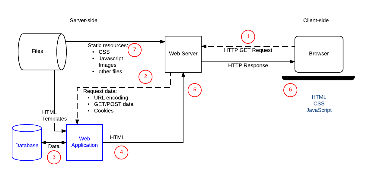
Overview of the request-response round-trip made from client to server and back again in a typical web application. Original source (with descriptions of each step): Anatomy of a dynamic request (MDN)
In a complete web application, sub-tasks can often be distributed between server and client sides in different ways. Traditionally, the server side takes care of heavy computations as well as functionalities that involve data that is not meant to be seen in its entirety. For example, databases are typically operated on the server side, for both of these reasons.
Server-side programs can be written in practically any programming language, including Python, and their architecture can be arbitrarily complex. On the other hand, client-side programs are typically run in web browsers which support a very restricted number of special-purpose languages:
- JavaScript, also known as ECMAScript (and having nothing to do with Java), is a general-purpose (Turing-complete) programming language for all kinds of client-side programs.
- HTML, HyperText Markup Language, is used for the content and structure on a web page.
- XML, eXtensible Markup Language, is a generalization of HTML also capable of storing structured data. (HTML is not strictly compliant with XML, but its later variant XHTML is. However, XHTML has not gained the popularity expected after the populatity of XML itself.)
- SVG, Scalable Vector Graphics, is another instance of XML, used for vector-based images on web pages. Other image types like PNG and JPG are formats, but not languages in the same way as SVG is.
- CSS, Cascading Style Sheets, is used for specifying the concrete layout and look of web pages on top of the content specified in HTML.
You can find excellent tutorials and references for all web technologies at the Mozilla Developer Network (MDN): https://developer.mozilla.org/en-US/docs/Web
9.1. HTTP
The Hypertext Transfer Protocol (HTTP) is the basic communication protocol of the web, designed to enable communications between clients and servers via requests and responses. A “protocol” just means an agreed-upon format. All HTTP messages are ultimately just plain-text strings, but they follow a particular format.
The examples below give a general idea, for more see: https://developer.mozilla.org/en-US/docs/Web/HTTP
Request
When a client sends a request to a server to http://example.com/cat , it might look something like this:
GET /cat HTTP/1.1
Host: example.com
User-Agent: Mozilla/5.0 (Macintosh; Intel Mac OS X 10_15_7) ...
Accept: */*
Made up of:
- a method:
GET(other methods includePOST,PATCH,DELETE, etc.) - a target:
/cat(path to resource on server) - a protocol version:
1.1 - headers: key-value pairs adding additional information to the request
There are many HTTP methods available as part of the protocol, but the most important ones are:
GET- retrieve a specific resource from the server
- optional arguments are sent in URL query
- should not modify data on the server
POST- send data to the server, creating or updating a resource
- arguments are sent in body of request
- can modify data on the server
Response
Similarly, a response has this format:
HTTP/1.1 200 OK
Content-Type: text/html; charset=UTF-8
Date: Fri, 21 Jun 2024 14:18:33 GMT
Last-Modified: Thu, 17 Oct 2019 07:18:26 GMT
Content-Length: 1234

<html>
<b>hello!</b>
</html>
Made up of:
- a protocol version:
1.1 - a status code and message:
200 OK(others include404 Not Foundand500 Internal Server Error) - headers: key-value pairs adding additional information to the response
- a blank line
- a body, which contains the actual payload of the response (in this example, some HTML code)
9.2. URLs
You surely already know what a URL is! URL stands for Uniform Resource Locator and are often just called a “web addresses”:
https://www.example.com/cat/?foo=bar+hex
You have likely already noticed that URLs have a very particular structure consisting of several parts. URLs have their own syntax, expressable by these simplified grammar rules:
<url>   ::= <scheme> :// <hostname> / <path> (? <query>)?
<query> ::= <attr> (& <attr>)*
<attr>  ::= <key> = <value>
Note that no spaces are allowed between the components (unlike most programming languages). A more complete description of URL structure can be found at: https://developer.mozilla.org/en-US/docs/Learn_web_development/Howto/Web_mechanics/What_is_a_URL
When working with standard formats such as URLs in your own code, it is typical to rely on an existing library rather than writing your own functions to process and/or generate these formats.
In the case of Python, we can use the standard library urllib.parse for analysing URLs:
>>> import urllib.parse
>>> urllib.parse.urlparse('https://www.example.com/cat/?foo=bar+hex')
ParseResult(
    scheme='https',
    netloc='www.example.com',
    path='/cat/',
    params='',
    query='foo=bar+hex',
    fragment=''
)
Thus we can easily pick out the parts of the URL we are interested in, without having to write our own string processing code.
The library can similarly help with generating URLs for us.
What happens when the query part needs to contain special characters such as space, ? or ä?
Such characters must be rewritten using an encoding in order to avoid breaking the URL structure.
This task is also taken care of by the urllib.parse library:
>>> base_url = 'https://www.example.com/cat'
>>> attrs = urllib.parse.urlencode({'foo': 'ser &trängen køn$t/g ut?'})
>>> base_url + '?' + attrs
'https://www.example.com/cat?foo=ser+%26tr%C3%A4ngen+k%C3%B8n%24t%2Fg+ut%3F'
Another library one can use for this is requests
which makes it particularly easy to make queries and extract answers from them (in addition to many other tasks related to web requests in general).
9.3. HTML
9.3.1. HTML syntax
Our goal is not to write HTML itself directly, but rather to analyse and generate HTML in Python. But first we need to understand its basic structure.
HTML is a “markup” language, meaning that it is essentially plain text with parts of it marked with tags. The b tag for instance means boldface, used as follows:
You must <b>check your code</b> before submitting it.
Note that there are start tags <b> and end tags </b> which must match, to delimit elements.
It is sometimes possible to leave out end tags, but this is not a good practice.
Attributes in start tags specify the element further.
A typical example is <a> (anchor), for links:
To learn more about HTML, see <a href="https://developer.mozilla.org/en-US/docs/Web/HTML">MDN's tutorials</a> which are very good.
More generally, the syntax of HTML can be expressed as follows (with only some of the recognised tag names included):
⟨element⟩   ::= ⟨starttag⟩ ⟨element⟩* ⟨endtag⟩
⟨starttag⟩  ::= <⟨tag⟩ ⟨attr⟩*>
⟨endtag⟩    ::= </⟨tag⟩>
⟨attribute⟩ ::= ⟨key⟩=⟨value⟩
⟨tag⟩       ::= html | head | body | title | ...
                     | h1 | h2 | ...
                     | a | b | p  ...
                     | ul | li | ...
                     | table | th | tr | td ...
9.3.2. Generating HTML
Consider now how to generate HTML programmatically. The idea is to use Python functions that at the same time force the result to be well-formatted. A simple example of such a function is:
def in_tag(tag, elem, attrs=''):
    return f'<{tag} {attrs}>{elem}</{tag}>'
By using in_tag to wrap some text in a tag, we will ensure that the opening and closing tag of an element always match.
This is basically the only thing it does, but in reality there are many other things to check if we want to ensure well-formed HTML:
- tag names must be valid (e.g.
<xyz>is not a valid HTML tag) - certain tags must have certain attributes (e.g.
<a>must always have ahrefattribute) - certain characters need escaping (e.g. text containing
<or attributes containing=)
Because of all these considerations, we typically would use a library which has been built for such a task and whose developers have hopefully thought of and tested all these edge cases. Some examples are htpy and Yattag.
9.3.3. Analysing HTML
We’ve seen how to generate HTML, but how about analysing it? For example, how can we find all links in a given web page? An HTML page is just a plain text file, or even just single long string of characters. So we could use some usual string processing to try and find all links:
def find_links(html):
    links = []
    pos = 0
    while True:
        # Find the next <a href="
        href_pos = html.find('<a href="', pos)
        if href_pos == -1: break
        start_quote = href_pos + len('<a href="')

        # Find the next "
        end_quote = html.find('"', start_quote)
        if end_quote == -1: break

        # Extract link and add
        links.append(html[start_quote:end_quote])
        pos = end_quote + 1
    return links
You can run this on a few simple examples and convince yourself that it works. Then you can try a few more examples and realise that there are many cases of valid HTML that this function won’t handle, for example:
- using single quotes (e.g.
<a href='www.example.com'>) - additional attributes (e.g.
<a title="link" href="www.example.com">) - unusual spacing (e.g.
<a\n\thref="www.example.com">)
As usual, instead of trying to think of and handle all these cases outselves, in many situations it makes more sense to use an existing library which is designed for exactly this task.
Popular examples include the Python standard library html.parser and BeautifulSoup.
9.4. XML
If you’re familiar with HTML, then understanding XML is fairly logical.
The main difference is that HTML is a language specifically designed for pages, and thus defines things such as a set of valid tags (<p>, <table>, etc) along with rules about their use (<a> must always have a href attribute, <ul> is not allowed inside of <p>, etc.)
The Extensible Markup Language (XML) is a generalisation of this, defining the structure based on tags with attributes, but enforcing little else. This makes it usable as a generic language for data modelling. We have mainly been using JSON as a data interchange format, which is the most popular format these days, but previously it was XML which was the main such format on the web. The rise of JSON in popularity correllates mainly with the rise of JavaScript itself as a language.
For example, this JSON data:
{
    "stops": {
        "Olskrokstorget": {
            "lat": 57.7146209,
            "lon": 11.9987871
        },
        "Svingeln": {
            "lat": 57.713358,
            "lon": 11.9917409
        }
    }
}
could equally well be encoded in XML as:
<stops>
  <stop>
    <name>Olskrokstorget</name>
    <lat>57.7146209</lat>
    <lon>11.9987871</lon>
  </stop>
  <stop>
    <name>Svingeln</name>
    <lat>57.713358</lat>
    <lon>11.9917409</lon>
  </stop>
</stops>
9.5. SVG
Scalable Vector Graphics (SVG) is an XML-based markup language for describing two-dimensional based vector graphics. So, an SVG file like this:
<svg width="190" height="160" xmlns="http://www.w3.org/2000/svg">
  <path
    d="M 10 80 C 40 10, 65 10, 95 80 S 150 150, 180 80"
    stroke="green"
    stroke-width="5"
    fill="transparent" />
</svg>
Would be rendered as:

As usual, a thorough tutorial and reference of SVG can be found at: https://developer.mozilla.org/en-US/docs/Web/SVG
9.5.1. Example: Modifying an SVG file
Let’s consider a concrete task: show shortest paths on the manually written Gothenburg tram map.

Gothenburg tram network SVG. Original source: https://commons.wikimedia.org/w/index.php?curid=92652381.
Since SVG is a kind of XML, we can use an XML parser library to process it.
In this case the standard library xml.etree.ElementTree.
Inspection of the SVG file shows that tramstop names are this kind of element:
<tspan
    sodipodi:role="line"
    x="253.33316"
    y="-23.96228"
    style="font-size:4.23333311px;stroke-width:0.26458332"
    id="tspan980-4-3-2-1-7-2-4-6-9">Chalmers</tspan>
Using tree recursion, our baseline algorithm can be:
- Get the list of stops in the desired shortest path.
- Traverse the XML element tree recursively:
- if the
textelement in the tree is in the list of stops, change the value of thestyleattribute to a larger font.
- if the
Implemented as follows:
import xml.etree.ElementTree as et

def color_xml_tree(tree, path):
    # check current node
    if tree.text in path:
        tree.attrib['style'] = "font-size:8px;fill:magenta"
    # recurse into children
    for child in tree:
        color_xml_tree(child, path)

MAP_FILE="Göteborgs_spårvägsnät.svg"
OUT_FILE="out.svg"
with open(MAP_FILE) as file:
    tree = et.fromstring(file.read())
color_xml_tree(tree, ["Chalmers", "Korsvägen", "Scandinavium"])
et.ElementTree(tree).write(OUT_FILE)
9.6. JavaScript
The web languages we’ve seen so far are all markup languages which describe content, but they are not fully-fledged programming languages that can do arbitraty computation, like Python. For mainly historical reasons, JavaScript is the only scripting language that web browsers run. So if you want to write code which runs on the client’s machine then you need to write it in JavaScript (or some other language which transpiles into it). Recently there is also WebAssembly, a low-level type of code similar to assembly which also runs in modern web browsers.
JavaScript shares some similarities with Python in that it is an interpreted, imperative general-purpose programming language. If you’re interested, you can see a comparison between JavaScript and Python. But we will not say anything more about JavaScript here. The main point is that web clients cannot run Python and thus we will not be looking at writing any client-side code as part of this course.
9.7. Web servers
What is a web server? It is essentially a program which runs forever, listening for HTTP requests from clients and sending responses back to them.
A basic web server can be written with the standard library http.server and might look something like this:
from http.server import BaseHTTPRequestHandler, HTTPServer

class HelloHandler(BaseHTTPRequestHandler):
    def do_GET(self):
        self.send_response(200)
        self.send_header('Content-type', 'text/plain')
        self.end_headers()
        self.wfile.write(b"Hello, World")

if __name__ == "__main__":
    server_address = ("localhost", 8000)
    httpd = HTTPServer(server_address, HelloHandler)
    httpd.serve_forever()
Run this code (note that it doesn’t terminate: it’s a server!) then visit http://localhost:8000 in your browser, and you will see a “Hello, World!” message. The HTTP response sent back to the client looks like this:
HTTP/1.0 200 OK
Server: BaseHTTP/0.6 Python/3.13.5
Date: Thu, 13 Nov 2025 08:18:55 GMT
Content-type: text/plain

Hello, World
What exactly is happening here? You are now running both a server and a client on the same computer! This is normal when developing web applications, that you run the server locally for testing purposes. But they are completely separate processes which communicate only via HTTP. This means that the client has no access to the code or any of the files which form part of the server program.
You could implement an entire web application using http.server, but since it is a very low-level library it would be rather tedious to do so.
Furthermore, the library documentation itself warns that:
http.server is not recommended for production. It only implements basic security checks.
So in the next section we will look at using a big industrial-strength web framework.
9.8. Web frameworks: Django
9.8.1. Introduction to Django
Most modern web development is done with frameworks, which bundle libraries, conventions, and some “magic” which in general make it quicker to develop a web application compared to doing it from scratch. There are countless frameworks out there, and their popularity changes over time. One of the most popular web frameworks for Python is Django, which we will use in this course and which you are very likely to come across in industry too.
Trying to understand all the things that a big framework does is often daunting, and you have to learn how to filter through the marketing speech:
Django is a high-level Python web framework that encourages rapid development and clean, pragmatic design. Built by experienced developers, it takes care of much of the hassle of web development, so you can focus on writing your app without needing to reinvent the wheel.
Quote from Djagno’s homepage https://www.djangoproject.com/
The features we are interested in are:
- HTTP server: listen to HTTP requests and send responses which are valid HTTP. We also want to handle concurrent requests from multiple clients efficiently.
- URL routing: handle different URLs in different ways, considering HTTP method, path, and queries.
- Serving static files: send certain files directly to client without any processing, such as images.
- Dynamic HTML templating: dynamically generate HTML pages with content specific for that request before sending to client.
- Form handling: automatically generate HTML forms and handle data submitted by them.
- Persistence to database: store and retrieve data from a database in a convenient way.
In order to use a framework, things must be done in the way the framework dictates. This means files need particular names in specific folders, functions need to have certain signatures, special base classes need to be inherited, etc. Everything we will see in the following sections is specific to how things are done in Django (version 5.2).
9.8.2. Models, views and templates
Many sources (although not Django itself, strangely) describe Django as following the Model-View-Template (MVT) design pattern. The idea is that there is a clear separation of concerns between different “layers” in the code:
-
Model (data layer): defines the structure of applications data and interacts with the database.
-
View (logic layer): handles the business logic, processing requests, managing data flow, and preparing data for display.
-
Template (presentation layer): combines static content with dynamic data using template to render content that is sent in responses.
In Django terms, we see that that these layers are reflected in the file structure. Consider a simple app which stores information about music bands and allows us to search for bands by name.
The model defines what our data objects look like:
# app/models.py
from django.db import models

class Band(models.Model):
    name = models.CharField(max_length=200)
    year = models.IntegerField()
The view handles requests, using input from the query to find the matching bands and combining this data with a template:
# app/views.py
from .models import Band
from django.shortcuts import render

def band_search(request):
    query = request.GET.get('query')
    matching_bands = Band.objects.filter(name__contains=query)
    return render(request, 'bands.html', {'bands': matching_bands})
The view is connected to a URL path using a URL pattern:
# app/urls.py
from django.urls import path
from . import views

urlpatterns = [
    path('bands/search/', views.band_search),
]
And our HTML template looks like this:
<!-- app/templates/bands.html -->
<h2>Search results:</h2>
<ol>

</ol>
All these parts work togther, so that when we send a GET request /bands/search/?query=Black we get something like the following rendered HTML as a response (assuming this data already exists in our data store):
<h2>Search results:</h2>
<ol>
    <li>The Black Crowes (started in 1984)</li>
    <li>The Black Keys (started in 2001)</li>
    <li>Black Sabbath (started in 1968)</li>
</ol>
9.8.3. Form handling
In our previous example we assumed that someone typed in the URL /bands/search/?query=Black directly, but usually such URLs are pieced together by the browser when a user submits a form.
A simple HTML form for this use case can look like this:
<form action="/bands/search/" method="GET">
    <label for="query_input">Query:</label>
    <input type="text" name="query" id="query_input" placeholder="Band name" />
    <input type="submit" value="Search" />
</form>
And is rendered visually like so:
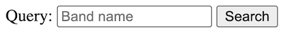
Notice that the details of the fields need to match the behaviour in our view: there is a single field with name q of type text.
It is entirely up to us to ensure that these things match.
We could just put this HTML directly into our template file and it should work, but Django offers functionality to automate the building of forms. To take advantage of this, we define the form in Django, making sure to inherit from the corresponding base class:
# app/forms.py
from django import forms

class BandSearchForm(forms.Form):
    query = forms.CharField(max_length=100)
This newly-defined form has a single field query of type CharField.
In order to render this form, we need to pass it to the template in our view. We’re going to update the behaviour of our view to work as follows:
- Show the form if there no search query, otherwise don’t show it
- Use the form’s inbuilt validation before accessing submitted data
# app/views.py
from .forms import BandSearchForm
from .models import Band
from django.shortcuts import render

def band_search(request):
    form = BandSearchForm(request.GET)
    if form.is_valid():
        query = form.data['query']
        matching_bands = Band.objects.filter(name__contains=query)
        return render(request, 'bands.html', {'bands': matching_bands})
    else:
        form = BandSearchForm()
        return render(request, 'bands.html', {'form': form})
Finally we just need to specify where in our template the form should go (note we still need to specify the enclosing <form> element ourselves):
<!-- app/templates/bands.html -->

<form action="/bands/search/" method="GET">

    <input type="submit" value="Search" />
</form>
9.8.4. Models and ORM
We’ve specified the structure of our data in app/models.py, but where does the data itself come from?
The answer is a database, which is not part of Django itself, but which Django interfaces with on our behalf.
Many database engines exist which usually run as standalone applications. In production environments they often run on different servers to the web server itself.
So-called “relational” databases (e.g. MySQL, PostgreSQL) use SQL (Structured Query Language) for interacting with them, but other kinds of databases exist which use different languages, such as MongoDB which uses a JavaScript-based query language.
The simplest database backend we can use with Django is SQLite,
which rather than being a separate application, stores all database contents inside a single local file.
One of the main features of Django is its object-relational mapper (ORM) which provides an interface between models as they are defined in Django, and the underlying database engine, without us having to write any SQL ourselves.
Django’s Model class (which our Band model inherits) allows us to add/update/find instances of our model directly through the class’ methods.
So, if we open up a Django shell we can add some new bands like so:
$ ./manage.py shell
>>> Band.objects.create(name="Dire Straits", year=1977)
<Band: Band object (1)>
>>> Band.objects.create(name="Pink Floyd", year=1965)
<Band: Band object (2)>
Although we have “only” created a few Python objects, in the background Django has taken care of persisting these objects into the database, by creating and running SQL queries like these:
INSERT INTO "app_band" ("name", "year") VALUES ('Dire Straits', 1977);
INSERT INTO "app_band" ("name", "year") VALUES ('Pink Floyd', 1965);
In fact we can peek inside our database using a separate SQL client to see that the data really is there:
$ sqlite3 db.sqlite3
sqlite> SELECT * FROM "app_band";
1|Dire Straits|1977
2|Pink Floyd|1965
Similarly, we can use Django’s ORM to filter entries in our database, in this case returning all objects where the year field is less than (year__lt) 1970:
>>> Band.objects.filter(year__lt=1970)
<QuerySet [<Band: Band object (2)>]>
To return this data, Django internally runs this SQL query on our database for us:
SELECT * FROM "app_band" WHERE "year" < 1970;
These are just a few simple examples of what Django’s ORM can do. As you can imagine, there are many features which cover things such as validation, relations between models, bulk updates, etc. In general ORMs are useful for a number of reasons:
- they take care of writing boilerplate code (converting from Python syntax to SQL and back), which is repetitive and error-prone,
- they add security by protecting against SQL injection attacks,
- they abstract away from the underlying database, making it easy to swap database engine without changing any code.
9.8.5. Migrations
Even though ORMs hide away lots of database details for us, there are still some situations which we need to understand and appreciate. We’ve seen about that the ORM automatically updates the contents of the database for us, but what about the structure of the database?
When defining a model in Django, before we can actually use it to add data, we need to ensure that the model structure as defined in Python is synced with the table structure in the database. That’s what migrations are for. First we need to create a migration:
$ ./manage.py makemigrations
Migrations for 'app':
  app/migrations/0001_initial.py
    + Create model Band
Then we need to apply the migration onto the database:
$ ./manage.py migrate
Operations to perform:
  Apply all migrations: admin, app, auth, contenttypes, sessions, tram
Running migrations:
  Applying app.0001_initial... OK
You might wonder why these steps need to be manual: why doesn’t Django just automatically update the structure of the database without needing these commands? The answer is to prevent data loss. Whenever changes are made to a model, we need to decide when those changes are applied onto the underlying database by creating and applying migrations using the steps above.
For example if we decide that Band.year field should be a date instead of an integer, we make this change in the model:
# app/models.py
from django.db import models

class Band(models.Model):
    name = models.CharField(max_length=200)
    year = models.DateField() # was previously IntegerField()
Then create a new migration:
$ ./manage.py makemigrations
Migrations for 'app':
  app/migrations/0002_alter_band_year.py
    ~ Alter field year on band
Then apply it:
$ ./manage.py migrate
Operations to perform:
  Apply all migrations: admin, app, auth, contenttypes, sessions, tram
Running migrations:
  Applying app.0002_alter_band_year... OK
These are boring details which would be nice to not have to think about. But the authors of Django have decided that it would be too unsafe to modify the database’s structure automatically as soon as you change the model. Therefore we have this migrations system, which adds a level of safety but also traceability when it comes to modifying the database’s structure, which is important for large applications in production.
9.8.6. Debugging a Django application
To debug a Django application in VS Code, follow these steps:
- Create a launch configuration:
- Either via the menu: Run → Add Configuration… → Python Debugger → Django, then specify the path to your
manage.pyfile. -
Or by adding a file
.vscode/launch.jsonin the root of your project with the following content, making sure to update the path to yourmanage.pyfile as necessary:{ "version": "0.2.0", "configurations": [ { "name": "Debug Django", "type": "debugpy", "request": "launch", "args": ["runserver"], "django": true, "autoStartBrowser": false, "program": "${workspaceFolder}/manage.py" } ] }
- Either via the menu: Run → Add Configuration… → Python Debugger → Django, then specify the path to your
- Once the launch configuration is created, you can start the debugger by going to Run → Start Debugging (keyboard shortcut F5).
- Once the server is running in debug mode, add a breakpoint inside your view and then make a request to the server (e.g. by reloading a page in the browser).
- The debugger will remain running until you exit it with the red stop button in the debug bar, or by killing the process with the trashcan button in the terminal.
9.8.7. A final word on frameworks
There are many things in Django which we haven’t seen, such as user authentication, caching, admin, internationalisation etc. which are outside the scope of this course. But we conclude with a quote on the potential downsides of choosing to use a big framwork such as Django:
Frameworks are powerful tools. We’d be lost without them. But there’s a cost to using them.
Using a framework requires a significant commitment. By accepting the framework into your code, you surrender your control over the details that the framework manages. Of course this seems like a good thing; and it usually is. However, there’s a trap waiting around the corner; and it’s hard to see it coming. Before you know it you find yourself engaged in all manner of unnatural acts, inheriting from its base classes, relinquishing more and more of the flow of control, bowing ever deeper to the framework’s conventions, quirks, and idiosyncrasies.
And yet despite the huge commitment you’ve made to the framework, the framework has made no reciprocal commitment to you at all. That framework is free to evolve in any direction that pleases its author. When it does, you realize that you are simply going to have to follow along like a faithful puppy.
Robert C. Martin (Uncle Bob), https://blog.cleancoder.com/uncle-bob/2014/05/11/FrameworkBound.html
10. The rest of Python
This chapter gives an overview of Python constructs that we have not yet seen but that will be needed to understand arbitrary Python code. The corresponding lecture will probably focus on just a few of them, whereas this chapter gives a more superficial overview of them all.
The following additional grammar rules complete the listing in Section 2.3:
<stm>  ::= ...
         | <decorator>* async? def <name> (<arg>,*) <rtyp>?: <block>
         | type <name> = <exp>
         | <exp> <typh> = <exp>
         | match <exp>: <case>+
         | await <exp>
<arg>  ::= ...
         | <name> <typh>
<case> ::= case <exp>: <stm>+
<typh> ::= : <exp>    # type hint
<rtyp> ::= -> <exp>   # return type
<exp>  ::= ...
         | <name> := <exp>
<op>   ::= ...
         | & | | | ^ | ~ | >> | <<
In addition to these new syntactic constructs, we will introduce regular expressions. From the point of view of Python grammar, they are just strings. But these strings are treated in a special way, so that they are actually a complex sublanguage of its own.
10.1 Type hints
Python is a dynamically typed language, which means that type checking is performed dynamically, at runtime. This is in contrast with static typing, which means that types are checked at compile time, before the program is executed. Dynamic typing has two main advantages:
- programs can be run and tested early
- functions and data structures can easily cover objects of different types
But is also has disadvantages:
- type errors in programs can remain undetected for a long time
- the argument and return types of functions are hard to specify precisely
This comic captures an essential difference between the two kinds of typing.
Most main-stream programming languages have static typing, which is considered necessary when programs are large and complex, and/or developed by different people at different times. Static type checking then gives a guarantee that different parts of the code match each other. Since the types are made explicit in the code by type signatures, programmers can communicate their intents to each other. Static typing also helps the compiler to generate more efficient machine code, because many machine instructions are specialized to types.
In order to get some of the advantages of static typing, Python has introduced type hints into the syntax of the language. These hints are, first of all, a good way to document the code. For example,
def take(n: int, s: str) -> str:
tells us that the take function takes an integer and a string as arguments and returns a string. It does not yet tell us what the function exactly does (it could, for instance, return the first n characters of the s), but it says much more than just
def take(n, s):
For this reason, type hints are getting more common in API documentation, where they are a both more compact and more precise way to document functions.
In addition to the documentation purpose, there are external tools that perform static type checking of Python code. A widely used such tool is mypy
This program can be run on the code file in the command line terminal. But also Visual Studio code has a type checker plug-in, called Pylance, which can be enabled as a part of the code development workflow.
10.2. The match statement
Commonly known also as “switch” in other languages, the match statement is used for pattern matching and allows us to rewrite chains of if/elif statements with a lot of useful features.
So the following if statement:
if status == 400:
    print("Bad request")
elif status == 404:
    print("Not found")
elif status == 418:
    print("I'm a teapot")
else:
    print("Unknown status")
can be rewritten into this match statement:
match status:
    case 400:
        print("Bad request")
    case 404:
        print("Not found")
    case 418:
        print("I'm a teapot")
    case _:
        print("Unknown status")
The improvement here may not be that great, it is mainly that we have avoided rewriting status == in each case.
More value is added when matching complex objects, such as lists. Here is a simple interpreter for string operators:
while True:
    command = input('> ')

    match command.split():
        case ['reverse', s]:
            print(s[-1::-1])
        case ['reverse', *s]:
            print('cannot reverse multiple words')
        case ['echo', *s]:
            print(*s)
        case ['square', s] if s.isdigit():
            print(int(s)**2)
        case ['quit'|'bye']:
            print('bye')
            break
        case _:
            print('try again')
But there are many more advanced things which you can do with pattern matching, see PEP 636 for more examples.
10.3. Assignment expression :=
The “Walrus” operator x := e assigns the value of e to x and returns it, which gives us a convenient way of rewriting this common pattern:
value = exp
if value:
    print(f"Value is: {exp}")
into this:
if value := exp:
    print(f"Value is: {value}")
The rationale of this is not only to save writing effort, but also to save computation, in case one is tempted to write
if exp:
    print(f"Value is: {exp}")
In this case, exp is evaluated twice, which can be an expensive operation. If exp has side effects (such as printing something or changing the value of an object), these are performed twice. This can sometimes be the desired outcome, but it can also result in a bug.
10.4. Binary numbers and bitwise operators: & | ^ ~ >> <<
Binary numbers can be given as literals prefixed with 0b and also converted from integers with the bin() function:
x = 0b101010

int(x)      # == 42
bin(42)     # == '0b101010'
Binary numbers can be combined with logical operations corresponding to and, or, xor (exclusive or), and not:
20 & 10     # == 0b10100 & 0b1010 == 0b0
20 | 10     # == 0b11110 == 30
20 ^ 10     # == 0b11110 == 30
~ 20        # == -21
Notice that the not-operation corresponds to the two’s complement encoding of negative numbers.
Another interesting pair of binary operations is shifts, which “move” the binary number left (adding zeros to the end, x << n = (x * (2**n)) or right (ignoring the last bits, x >> n= (x // (2**n))):
10 << 2    # 40
10 << 3    # 80

100 >> 2   # 25
101 >> 2   # 25
Shifts provide an efficient way to multiply an divide by powers of 2, which is exploited in optimizing compilers.
10.8. Asynchronous I/O
Asynchronous programs are programs running at the same time without blocking each other. Python provides the keyword async for the definition of asynchronous functions, and await for pausing the execution of a program. The standard library asyncio adds several functionalities to work with such programs.
This course does not cover asynchronous programs, but we just show here a minimal example that you can try:
import asyncio

async def hello(i, n):
    print(f"hello {i} started, going to sleep for {n} seconds")
    await asyncio.sleep(n)
    print(f"hello {i} done")

async def main():
    task1 = asyncio.create_task(hello(1, 4))
    task2 = asyncio.create_task(hello(2, 6))
    await task1
    await task2

asyncio.run(main())
For more details, see the asyncio module.
10.7. Regular expressions
Regular expressions are patterns that are used for matching strings. They are actually a special case of grammar rules, corresponding to so-called regular languages, whereas the grammar rules used in this document cover a wider set of context-free languages.
Standard regular expressions are formed by the following operators, where we use the variables A and B to denote the regular expressions that are combined:
| expression | name | matches |
|---|---|---|
| a | symbol | character a |
| A B | sequence | A followed by B |
| A | B | union | A or B |
| A? | optional | zero or one A |
| A* | Kleene star | zero or more A |
| A+ | Kleene plus. | one or more A |
| . | any | any character (except newline) |
For example, the regular expression (P|p).* matches any string that starts with P or p.
Python has a wide range of regular expression syntax extensions, documented here. Here is an example for matching sequences of digits:
dig = re.compile(r"\d+")
The expression \d matches single digits. The regular expression itself is given in a raw string, prefixed with r, preventing the interpretation of backslashes as excapes. This raw string is given as an argument to re.compile(), which converts the expression into a data structure called finite automaton. It is this automaton that is used for the actual matching with regular expressions. Thus the following piece of code reads a file and prints all numbers (sequences of digits) that occur in it:
with open(filename) as file:
    for line in file:
        peint(dig.findall(line))
The following expression can be used for matching URLs:
r"http[s]?://[\S]+"
This is a simplification: it matches all strings starting with http or https followed by :// followed by one or more non-space characters. A more accurate expression takes care checking that it follows the ruls for a valid URL:
(?i)\b((?:[a-z][\w-]+:(?:/{1,3}|[a-z0-9%])|www\d{0,3}[.]|[a-z0-9.\-]+[.][a-z]{2,4}/)(?:[^\s()<>]+|\(([^\s()<>]+|(\([^\s()<>]+\)))*\))+(?:\(([^\s()<>]+|(\([^\s()<>]+\)))*\)|[^\s`!()\[\]{};:'".,<>?«»“”‘’]))
This expression is from here.
Learning the full syntax of Python’s regular expressions and their productive use would probably need almost a full course of its own.
A. Appendix: Git version control system
-
When we save a file on our computer, the previous version of it is overwritten and basically lost forever. This means we only ever have the most recent version of it.
-
What happens when we are a team of developers who all want to work on the same codebase? Sending files around quickly becomes tedious.
Git is a tool which address both of these issues. By storing our code inside a repository, we get:
- Versioning: maintaining a history of file changes which we access at any time
- Collaboration: allowing multiple developers to work on the same code and combine their individual changes
Basic use of Git requires understanding of the following concepts, which we will explain in the subsequent sections:
- diffs
- staging
- committing
- pushing/pulling, remotes
- merging and conflicts
A.1. Setting up
First a repository must be created somewhere. This could be done on our computer, but in the case of this course, repositories for each lab will be created for us on GitLab. Can can then clone the repository locally onto our computer via its URL with something like:
$ git clone git@git.chalmers.se:cajohn/dummy.git
This copies the repository (with all its history) into a local folder, by default with same name as repository, e.g. dummy
A.2. Making local changes
Now the files in the repository are on our machine, we can view and edit them as usual using for example VS Code.
Let’s say our repository contains a single file hello.py with the following contents:
def hello(name):
    ... # TODO
We then open the file, add a reasonable implementation for our function, and save it, so that now our updated file looks like this:
def hello(name):
    print(f"Hello {name}!")

hello("Dolly")
A.3. Diffs
When we save a file, that local file is overwritten as usual.
At this point, our version of hello.py (the one in our working tree) has diverged from the version that is in the repository.
We can view a comparison of what has changed (known as a diff) with the command git diff which gives the output:
diff --git a/hello.py b/hello.py
index d289827..a348ee6 100644
--- a/hello.py
+++ b/hello.py
@@ -1,2 +1,4 @@
 def hello(name):
-    ... # TODO
+    print(f"Hello {name}!")
+
+hello("Dolly")
This view shows what has changed in our local version of the file, compared to the version in the repository. The diff tells us that one line was removed and three new ones added.
To get a summary of which files have changed, use:
$ git status
On branch main
Changes not staged for commit:
  (use "git add <file>..." to update what will be committed)
  (use "git restore <file>..." to discard changes in working directory)
    modified:   hello.py

no changes added to commit (use "git add" and/or "git commit -a")
To save these changes in our repository (not the same thing as saving a file), we need to commit them.
A.4. Staging
What exactly should we commit? This is something we have to tell Git explicitly, known as staging. Tell Git to stage all the changes in a specific file with:
$ git add hello.py
We can also stage all changes across all changed files with git add . but this is often too blunt and easily leads to adding things into our repo which we don’t want.
Now if we check the status again, we see that our changes are staged (but not yet committed):
git status
On branch main
Changes to be committed:
  (use "git restore --staged <file>..." to unstage)
    modified:   hello.py
A.5. Committing
Now we can finally commit our staged changes by creating a commit as follows:
$ git commit -m "Implement hello function"
[main eab9fc4] Implement hello function
 1 file changed, 3 insertions(+), 1 deletion(-)
Note that all commits must include a message (that’s what the -m flag specifies).
We should always give our commits meaningful but short messages!
A good tip is to always start with a verb, e.g. “add”, “fix”, “update”, etc.
Note our new commit has been given a unique identifier eab9fc468247040f9352736d20762aa00a4eb769 called a SHA (from “Secure Hash Algorithm”). SHAs are always 40 characters long, but you will often see them abbreviated to the first 7-8 characters for convenience, as eab9fc4 above.
Now we have committed the code to our repository, so there is no longer any diff (git diff gives empty output) and our repository status has also updated accordingly:
$ git status
On branch main
nothing to commit, working tree clean
We can see a history of all commits, including the one we just created, with git log:
commit eab9fc468247040f9352736d20762aa00a4eb769 (HEAD -> main)
Author: John J. Camilleri <john.j.camilleri@chalmers.se>
Date:   Wed Oct 29 11:21:40 2025 +0100

    Implement hello function

commit a5a311ccd78c285f9292c8c0c037659e37d376c3
Author: John J. Camilleri <john.j.camilleri@chalmers.se>
Date:   Wed Oct 29 10:58:27 2025 +0100

    Add hello template
A.6. Pushing
Note that even after committing our code, this new commit only exists locally (in the copy of the repository on our computer). That commit will not automatically appear in any other copies of the repository (remotes), such as on GitLab.
In order to sync our local repository with a remote one, we need to push our commits to it. In the simplest case, it goes like this:
$ git push
Enumerating objects: 9, done.
Counting objects: 100% (9/9), done.
Delta compression using up to 12 threads
Compressing objects: 100% (4/4), done.
Writing objects: 100% (9/9), 803 bytes | 803.00 KiB/s, done.
Total 9 (delta 0), reused 0 (delta 0), pack-reused 0 (from 0)
remote: MAX: 1500000, CURRENT: 116
To git.chalmers.se:cajohn/dummy.git
 * [new branch]      main -> main
branch 'main' set up to track 'origin/main'.
A.7. Pulling
Similarly, if changes have been made to the remote version of our repository, e.g. by our partner pushing to it, those changes do not automatically appear on our machine. In order to sync, we will need to pull from that remote into our local copy. If there are no remote changes to be pulled, we will simply see:
$ git pull
Already up to date.
If however there are some changes to be synced, we might see something like the following:
$ git pull
remote: Enumerating objects: 4, done.
remote: Counting objects: 100% (4/4), done.
remote: Compressing objects: 100% (3/3), done.
remote: Total 3 (delta 0), reused 0 (delta 0), pack-reused 0 (from 0)
Unpacking objects: 100% (3/3), 330 bytes | 165.00 KiB/s, done.
From git.chalmers.se:cajohn/dummy
   eab9fc4..6dce3ed  main       -> origin/main
Updating eab9fc4..6dce3ed
Fast-forward
 README.md | 3 +++
 1 file changed, 3 insertions(+)
 create mode 100644 README.md
In this case we see that a new file README.md has been added to our repository.
After pulling, we can now access that file locally.
A.8. Diverging changes
As you should have already noticed, the different copies of the repository (on our computer, on our partner’s computer, and on GitLab) are not automatically kept in sync. Changes can happen in these different copies at the same time, and there is no master copy of the repository which always has the most up-to-date version of things. This is what it means to be distributed.
It is only when syncing (pushing/pulling) with another copy of the repository (a remote) that we will become aware of potential changes that have happened elsewhere. Despite being fully distributed, in practice we almost always sync our repositories with the same server (in our case GitLab) and never between “peers”, i.e. directly with our partner’s computer. But this is just a convention, not a limitation of Git.
When syncing changes with a remote copy of the repository, there are different scenarios which might arise. Firstly if the remote has changes which we don’t have, we must first pull those changes to our copy before we can push.
- If we haven’t made any commits since the last pull:
- If we haven’t made any changes to our working copy, the incoming commits from the remote are pulled and applied immediately in a fast-forward.
- If we have made changes to our working copy, but they don’t overlap with the incoming commits, then they also be applied in a fast-forward. Our local changes to working copy will remain untouched.
- If we have made changes to the working copy, and they do overall with the incoming commits, the pull will fail. In this case we can commit our changes or temporarily stash them before trying to pull again.
- If we have made commits which aren’t yet pushed, our changes will need to merged together with the incoming ones, in order to unify the diverging versions.
- Git will try to automatically merge our code, which will succeed if the changes don’t overlap. It will usually ask us to specify a commit message for this new merge commit, but we can accept the default.
- If the changes overlap and an automatic merge is not possible, we will warned that we have conflicts that need to be resolved manually (see the next section about this).
As you can see, it can get a bit involved, and in reality things can get even more complicated than this. But it’s most important to understand the basics at this point.
A.9. Merge conflicts
Consider that our hello.py file currently looks like this:
def hello(name):
    print(f"Hello {name}!")

hello("Dolly")
Let’s say I change the name to "Jerry":
def hello(name):
    print(f"Hello {name}!")

hello("Jerry")
and then commit these changes:
$ git add hello.py
$ git commit -m "Change name to Jerry"
[main 6c24e36] Change name to Jerry
 1 file changed, 1 insertions(+), 1 deletion(-)
Now I want to push my changes to the remote:
$ git push
To git.chalmers.se:cajohn/dummy.git
 ! [rejected]        main -> main (fetch first)
error: failed to push some refs to 'git.chalmers.se:cajohn/dummy.git'
hint: Updates were rejected because the remote contains work that you do not
hint: have locally. This is usually caused by another repository pushing to
hint: the same ref. If you want to integrate the remote changes, use
hint: 'git pull' before pushing again.
hint: See the 'Note about fast-forwards' in 'git push --help' for details.
But the push fails because there are new commits which I haven’t pulled yet. This probably happened because my partner also made some changes and has already pushed them to the remote. So we need to pull these changes first before we can push:
$ git pull
remote: Enumerating objects: 5, done.
remote: Counting objects: 100% (5/5), done.
remote: Compressing objects: 100% (3/3), done.
remote: Total 3 (delta 0), reused 0 (delta 0), pack-reused 0 (from 0)
Unpacking objects: 100% (3/3), 324 bytes | 108.00 KiB/s, done.
From git.chalmers.se:cajohn/dummy
   6dce3ed..246add2  main       -> origin/main
Auto-merging hello.py
CONFLICT (content): Merge conflict in hello.py
Automatic merge failed; fix conflicts and then commit the result.
However this also fails. Git is unable to automatically merge our changes together because they affect the same part of the file (as described in 2.2 above). We now have a merge conflict in hello.py which we need to resolve manually.
$ git status
On branch main
Your branch and 'origin/main' have diverged,
and have 1 and 1 different commits each, respectively.
  (use "git pull" if you want to integrate the remote branch with yours)

You have unmerged paths.
  (fix conflicts and run "git commit")
  (use "git merge --abort" to abort the merge)

Unmerged paths:
  (use "git add <file>..." to mark resolution)
    both modified:   hello.py

no changes added to commit (use "git add" and/or "git commit -a")
The working copy of hello.py now looks like this:
def hello(name):
    print(f"Hello {name}!")

<<<<<<< HEAD
hello("Jerry")
=======
hello("Elaine")
>>>>>>> 246add2b0b269de9f5405bdd8a048fdde0fce2d6
Now we must edit the file manually, removing the conflict markers and deciding how to resolve this conflict, maybe like so:
def hello(name):
    print(f"Hello {name}!")

hello("Jerry and Elaine")
Now all that remains is to:
-
Mark the conflict as resolved:
$ git add hello.py -
Complete the merge commit:
$ git commit [main 3564ff7] Merge branch 'main' of git.chalmers.se:cajohn/dummy -
Push the new commit (the merge commit) to our remote:
 $ git push
 Enumerating objects: 10, done.
 Counting objects: 100% (10/10), done.
 Delta compression using up to 12 threads
 Compressing objects: 100% (6/6), done.
 Writing objects: 100% (6/6), 672 bytes | 672.00 KiB/s, done.
 Total 6 (delta 1), reused 0 (delta 0), pack-reused 0 (from 0)
 remote: MAX: 1500000, CURRENT: 220
 To git.chalmers.se:cajohn/dummy.git
 246add2..3564ff7  main -> main
This was a relatively simple case, and in practice resolving merge conflicts can be a lot more involved. But, it is an inevitable result of having a distributed system like Git, and something you need to be aware of.
A.10 Advanced Git use
We have covered the basics needed for working collaboratively with Git. As you might imagine, there are many more features and uses which we haven’t covered. Some of the most common ones are mentioned briefly below:
- Branches allow us to have multiple versions of our code inside the same repository and switch easily between them, and are often used to give developers their own isolated space to work on some feature without having their commits conflict with everyone else’s.
- Tags provide a way of uniquely labeling commits in a repository. In this course, they will be used for indicating submissions.
- Merge requests are not a feature of Git itself, bur rather of the GitLab platform (on GitHub they are called “pull requests”). They add extra functionality around merging branches together, such as the ability to have discussions on the diff itself. In this course, merge requests are used as part of the submission and grading process.
- Forks are conceptually similar to branches, in that they allow you to work on a diverging copy of a codebase. However like merge requests, they are not a feature of Git itself but of platforms like GitLab and GitHub, and exist mainly to allow developers to contribute to projects without needing to be given explicit access to the original repository.
As always, the best way to learn more is to consult the official documentation:
- Official book: https://git-scm.com/book/en/v2
- Detailed reference: https://git-scm.com/docs
- Cheat sheet: https://git-scm.com/cheat-sheet